
Normal Distribution and Geometric Construction
Loading the math board and drawing, please wait…
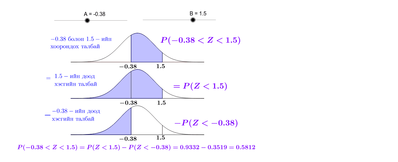
This example demonstrates the normal distribution curve and its geometric properties, integrating elements like straight lines, special points, and integers for visualization. Core concepts include normal distribution, line equations, special point calculations, integer sets, circumcircle, and tangent lines. GeoGebra commands and objects such as Function, Segment, Vector, Integral, and LPX2 are used in the construction. Suitable for high school and above mathematics education, showcasing the intersection of probability statistics and analytical geometry.
GeoGebra Commands & Parameters
Function(g(x) + Lv2, -4, 4) → Bell2Function(g(x) + Lv3, -4, 4) → Bell3Segment(((-4), Lv1), (4, Lv1)) → xaxsg1Vector((0, 0), (1, 0)) → UntXIntegral(g, A, B) → BtwArIntegralBetween(Bell3, Lv3, -4, A) → LTAArIntegralBetween(Bell2, Lv2, -4, B) → LTBArFunction(g, -4, 4) → Bell1Segment(((-4), Lv2), (4, Lv2)) → xaxsg2Segment(((-4), Lv3), (4, Lv3)) → xaxsg3Segment((A, Lv1), (A, Bell1(A))) → vrtA1Segment((B, Lv1), (B, Bell1(B))) → vrtB1Segment((B, Lv2), (B, Bell2(B))) → vrtB2Segment((A, Lv2), (A, Bell2(A))) → vrtA2Segment((A, Lv3), (A, Bell3(A))) → vrtA3Segment((B, Lv3), (B, Bell3(B))) → vrtB3
AI Drawing Prompt Reference
Draw a horizontal line spanning from -4 to 4, with two parallel lines above and below it in different colors. Sketch a symmetric bell-shaped curve in the center to represent the normal distribution. Mark the intersection points of the curve with the horizontal line and connect them with straight lines to the corresponding points on the curve. Finally, add vertical lines at both ends of the horizontal line, connecting them to the top and bottom intersection points on the bell-shaped curve to create a geometric structure.
The prompt above was compiled from the original drawing commands and is for reference only.