Normal Distribution as the Limit of the Binomial

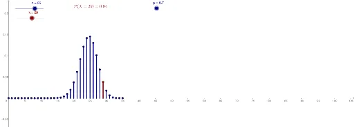
This GeoGebra example dynamically illustrates how the binomial probability mass function approaches the normal distribution curve as the number of trials n increases, demonstrating the classical limit phenomenon central to the Central Limit Theorem. The core mathematical concepts involve binomial distribution, normal distribution, continuity of probability distributions, and the approximation of discrete distributions by continuous ones. The construction uses the Sequence command to generate a series of points, Element and Segment commands to connect adjacent points into a polyline, and sliders for n, k, and p to control the number of trials, success count, and success probability. Additional objects like kPoint, kSeg, and text1 highlight specific points, segments, and parameter values. This resource is ideal for high school or undergraduate statistics courses when teaching the normal approximation to the binomial distribution or the Central Limit Theorem, providing an intuitive visual bridge between discrete and continuous probability models.