
Normal Curves
Loading the math board and drawing, please wait…
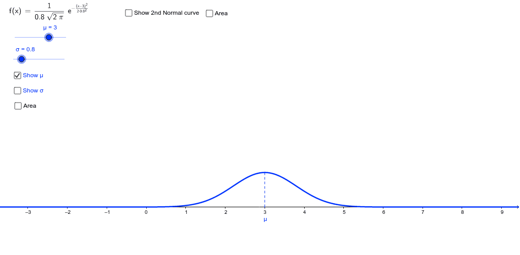
This example demonstrates normal distribution curves, mean, standard deviation, and the area within an interval. Key mathematical concepts include normal distribution, statistics, and probability. Using GeoGebra commands such as Segment, Point, and Integral, users can dynamically adjust the mean and standard deviation to observe their effects on the curve. Suitable for high school and above students learning probability and data analysis.
GeoGebra Commands & Parameters
Segment((μ, 0), (μ, f(μ))) → aSegment((x(A), 0), A) → cSegment(B, (x(B), 0)) → dSegment((μ_1, 0), (μ_1, f_1(μ_1))) → a_1Segment((x(A_1), 0), A_1) → c_1Segment(B_1, (x(B_1), 0)) → d_1Point(xAxis) → GIntegral(f, x(D), x(G)) → jPoint(xAxis) → HPoint(xAxis) → IIntegral(f_1, x(H), x(I)) → lLaTeX(f, true, true) → text1Sequence(RandomNormal[6.2, 3], k, 1, 100) → list2
AI Drawing Prompt Reference
Draw a normal distribution curve with mean μ and standard deviation σ. Mark the mean point μ on the x-axis and a movable point A. Draw a vertical line from A to the curve and calculate the area under the curve from μ to A. Then, change the mean and standard deviation, repeat the process, and observe the changes. Finally, display the formula of the normal distribution function.
The prompt above was compiled from the original drawing commands and is for reference only.