
Live Regression
Loading the math board and drawing, please wait…
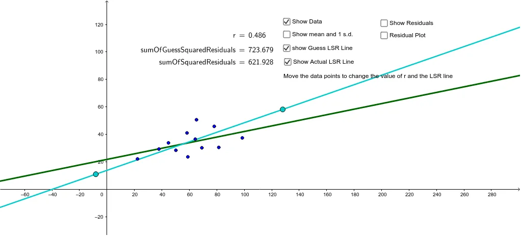
This example demonstrates how moving data points can affect the linear regression line. Key mathematical concepts include linear regression, correlation coefficient, and residual analysis. Construction involves calculating means, standard deviations, and using GeoGebra commands like MeanX, MeanY, SampleSDY, and ResidualPlot. Suitable for high school students or college freshmen in statistics learning and practice.
GeoGebra Commands & Parameters
MeanX(dataList) → xbarMeanY(dataList) → ybarSampleSDY(dataList) → s_ySampleSDX(dataList) → s_xPMCC(dataList) → rResidualPlot(dataList, f) → residualPointsSequence(y(Element[residualPoints, k]), k, 1, 12) → residualsElement(x(dataList), A1) → B1Element(y(dataList), A1) → C1Element(x(dataList), A2) → B2Element(y(dataList), A2) → C2Element(x(dataList), A3) → B3Element(y(dataList), A3) → C3Element(x(dataList), A4) → B4Element(y(dataList), A4) → C4Element(x(dataList), A5) → B5Element(y(dataList), A5) → C5Element(x(dataList), A6) → B6Element(y(dataList), A6) → C6Element(x(dataList), A7) → B7Element(y(dataList), A7) → C7Element(x(dataList), A8) → B8Element(y(dataList), A8) → C8Element(x(dataList), A9) → B9Element(y(dataList), A9) → C9Element(x(dataList), A10) → B10Element(y(dataList), A10) → C10Element(x(dataList), A11) → B11Element(y(dataList), A11) → C11Element(x(dataList), A12) → B12Element(y(dataList), A12) → C12Sequence(Segment[Element[dataList, k], (x(Element[dataList, k]), f(x(Element[dataList, k])))], k, 1, 12) → residualSegmentsSequence(y(Element[dataList, k]) - g(x(Element[dataList, k])), k, 1, 12) → residualsOfGuessSum(residualsOfGuess) → sumOfGuessResidualsSequence(Element[residualsOfGuess, k]^(2), k, 1, 12) → squaresOfGuessResidualsSum(squaresOfGuessResiduals) → sumOfGuessSquaredResidualsLaTeX(r, true, true) → text1Sequence(Element[residuals, k]^(2), k, 1, 12) → squaresOfResidualsSum(squaresOfResiduals) → sumOfSquaredResidualsSum(residuals) → sumOfResidualsLaTeX(sumOfGuessSquaredResiduals, true, true) → text2LaTeX(sumOfSquaredResiduals, true, true) → text3
AI Drawing Prompt Reference
Create a linear regression plot showing how moving data points affects the regression line. Include data points and the fitted line, with mean, standard deviation, and residuals labeled. Use different colors or shapes for residuals, and display the sum of squared residuals and correlation coefficient values. Start with data points and the regression line, then calculate and show residuals and their squares, finally label key statistics.
The prompt above was compiled from the original drawing commands and is for reference only.