
Monge Projection of the Cube
Loading the math board and drawing, please wait…
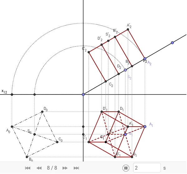
① This example demonstrates how to obtain the top view and front view of a cube using Monge (orthographic) projection when the plane, centre, and a vertex of one face are known. ② Core mathematical concepts include orthographic projection in solid geometry, the principles of Monge projection in descriptive geometry, spatial vectors and plane relationships, and the geometric properties of projection transformations. ③ Construction highlights: the GeoGebra commands Point, Ray, OrthogonalLine, Segment, Mirror, Intersect, Line, Circle, CircleSector, CircleArc are employed to create objects such as x12, A, B, β2, S2, A2, b, c, S1, A1, d, e, C1, a, C2, f, a4, g, h, i, So, Ao, k, p, p3, A0, A02, r3, j, q3, S0, s3, F, G, c4, t3, l, C0, n, q, using rays, perpendicular lines, segments, reflections, intersections, and circular arcs to build the two projection planes. ④ Suitable for high‑school solid geometry and university descriptive geometry courses, as well as for geometric construction practice and understanding projection transformations.
GeoGebra Commands & Parameters
Point(x_{12}) → BRay(B, A) → β_2Point(β_2) → S_2Point(β_2) → A_2OrthogonalLine(S_2, x_{12}) → bOrthogonalLine(A_2, x_{12}) → cPoint(b) → S_1Point(c) → A_1Segment(S_2, S_1) → dSegment(A_2, A_1) → eMirror(A_1, S_1) → C_1OrthogonalLine(C_1, x_{12}) → aIntersect(a, β_2) → C_2Segment(C_1, C_2) → fSegment(A_1, C_1) → a_4Line(S_1, x_{12}) → gLine(A_1, x_{12}) → hOrthogonalLine(B, x_{12}) → iIntersect(g, i) → S_oIntersect(h, i) → A_oCircle(S_o, Segment[B, S_2]) → kCircle(A_o, Segment[B, A_2]) → pCircle(B, A_2) → p_3Intersect(p, h, 1) → A_0Intersect(p_3, x_{12}, 1) → A_{02}CircleSector(B, A_2, A_{02}) → r_3Segment(A_0, A_1) → jSegment(A_{02}, A_0) → q_3Intersect(k, g, 1) → S_0Circle(B, S_2) → s_3Intersect(s_3, x_{12}) → F, GCircleArc(B, S_2, F) → c_4Segment(F, S_0) → t_3Segment(S_0, S_1) → lMirror(A_0, S_0) → C_0Segment(A_0, C_0) → nOrthogonalLine(S_0, n) → qCircle(S_0, C_0) → rIntersect(r, q, 2) → D_0Intersect(r, q, 1) → B_0Segment(B_0, D_0) → sSegment(A_0, B_0) → tSegment(B_0, C_0) → a_1Segment(C_0, D_0) → b_1Segment(D_0, A_0) → c_1OrthogonalLine(B_0, i) → d_1Segment(C_0, C_1) → mOrthogonalLine(D_0, i) → e_1Intersect(i, e_1) → D_oIntersect(i, d_1) → B_oCircle(B, Segment[D_0, D_o]) → f_1Intersect(f_1, β_2, 1) → D_2OrthogonalLine(D_2, x_{12}) → g_1Intersect(e_1, g_1) → D_1Segment(D_0, D_1) → h_1Segment(D_1, D_2) → i_1Circle(B, Segment[B_0, B_o]) → k_1Intersect(k_1, β_2, 1) → B_2OrthogonalLine(B_2, x_{12}) → j_1Intersect(d_1, j_1) → B_1Segment(B_0, B_1) → l_1Segment(B_1, B_2) → m_1Segment(B_1, A_1) → n_1Segment(A_1, D_1) → p_1Segment(D_1, C_1) → q_1Segment(C_1, B_1) → r_1Segment(B_1, D_1) → s_1Segment(A_1, C_1) → t_1OrthogonalLine(C_2, β_2) → a_2OrthogonalLine(B_2, β_2) → b_2OrthogonalLine(S_2, β_2) → c_2OrthogonalLine(D_2, β_2) → d_2OrthogonalLine(A_2, β_2) → e_2Circle(S_2, Segment[A_0, B_0]) → f_2Intersect(f_2, c_2, 2) → S'_2OrthogonalLine(S'_2, c_2) → g_2Intersect(a_2, g_2) → C'_2Intersect(b_2, g_2) → B'_2Intersect(d_2, g_2) → D'_2Intersect(e_2, g_2) → A'_2Segment(C_2, C'_2) → h_2Segment(B_2, B'_2) → i_2Segment(D_2, D'_2) → j_2Segment(A_2, A'_2) → k_2Segment(A'_2, C'_2) → l_2OrthogonalLine(A'_2, x_{12}) → m_2OrthogonalLine(D'_2, x_{12}) → n_2OrthogonalLine(S'_2, x_{12}) → p_2OrthogonalLine(B'_2, x_{12}) → q_2OrthogonalLine(C'_2, x_{12}) → r_2Intersect(r_2, m) → C'_1Intersect(q_2, d_1) → B'_1Intersect(p_2, g) → S'_1Intersect(n_2, e_1) → D'_1Intersect(m_2, h) → A'_1Segment(C'_2, C'_1) → s_2Segment(B'_2, B'_1) → t_2Segment(S'_2, S'_1) → a_3Segment(D'_2, D'_1) → b_3Segment(A'_2, A'_1) → c_3Segment(D_1, D'_1) → d_3Segment(S_1, S'_1) → e_3Segment(C_1, C'_1) → f_3Segment(B_1, B'_1) → g_3Segment(A_1, A'_1) → h_3Segment(D'_1, C'_1) → i_3Segment(C'_1, B'_1) → j_3Segment(B'_1, A'_1) → k_3Segment(B'_1, D'_1) → l_3Segment(C'_1, A'_1) → m_3Segment(D'_1, A'_1) → n_3Intersect(r_3, x_{12}, 1) → CIntersect(r_3, x_{12}, 1) → DIntersect(r_3, s_3, 1) → E