
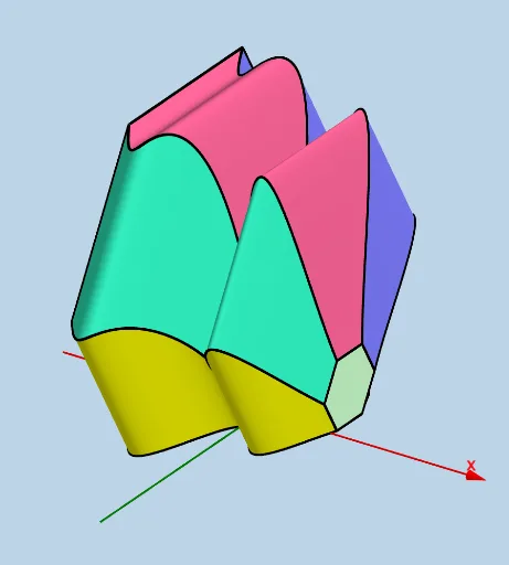
Modifiable Solid: Regular Hexagon Cross Sections Parallel to yAxis
Loading the math board and drawing, please wait…
This example demonstrates a modifiable solid where cross sections parallel to the yAxis are regular hexagons. Key math concepts include coordinate geometry and calculus-based cross-section analysis. Construction highlights the use of commands and objects like Segment, Midpoint, Intersect, Line, Sphere, Textfield, Rotate, Polygon, CurveCartesian, and Surface in GeoGebra. Suitable for high school and above students learning the relationship between solid geometry and function graphs.
GeoGebra Commands & Parameters
Segment(H, I) → s_1Midpoint(s_1) → A_1Segment(J, K) → q_1Midpoint(q_1) → ZMidpoint(s_1) → EMidpoint(q_1) → FIntersect(upper, h, (0, 8)) → BIntersect(lower, h, (0, -4)) → CSegment(C, B) → qIntersect(upper, q, (0, 8)) → GMidpoint(C, G) → TLine(B, D) → iSphere(B, d) → eSegment(C, B) → pTextfield(upper) → InputBox1Textfield(lower) → InputBox2Textfield(a) → InputBox3Textfield(b) → InputBox4Segment(C, G) → k_1Line(C, G) → jSphere(G, T) → kLine(T, T + (1, 0, 0)) → mRotate(G, pi / 3, F_1, m) → G'Rotate(G', pi / 3, F_1, Line[F_1, F_1 + (1, 0, 0)]) → G''Line(F_1, F_1 + (1, 0, 0)) → nRotate(G'', pi / 3, F_1, n) → G'''Rotate(G''', pi / 3, F_1, n) → G_1Polygon(C, G, G', G'', G''', G_1) → poly1, c_1, g_2, g', g'', g''', g_3Segment(G', G'') → lSegment(G'', G''') → rSegment(G''', G_1) → sSegment(G_1, C) → tSegment(G', G) → i_1Line(Z, Z + (1, 0, 0)) → fLine(D_1, D_1 + (1, 0, 0)) → gRotate(J, pi / 3, D_1, g) → J'Rotate(J', pi / 3, D_1, g) → J''Rotate(J'', pi / 3, D_1, g) → J'''Rotate(J''', pi / 3, D_1, g) → E_1Segment(J, J') → f_1Segment(J', J'') → g_1Segment(J'', J''') → j_1Segment(J''', E_1) → n_1Segment(E_1, K) → p_1Line(H_1, H_1 - (1, 0, 0)) → l_1Rotate(I, pi / 3, H_1, l_1) → I'Rotate(I', pi / 3, H_1, l_1) → I''Rotate(I'', pi / 3, H_1, l_1) → I'''Rotate(I''', pi / 3, H_1, l_1) → I_1Segment(I, I') → m_1Segment(I', I'') → r_1Segment(I'', I''') → a_1Segment(I''', I_1) → b_1Segment(I_1, H) → d_1Polygon(H, I, I', I'', I''', I_1) → poly2, h_2, i_2, i', i'', i''', i_3Polygon(K, J, J', J'', J''', E_1) → poly3, k_2, j_2, j', j'', j''', e_1CurveCartesian(t, (0.5 * (lower(t) + upper(t))) - (upper(t) - lower(t)), (((-sqrt(3))) / 2 * (lower(t) - upper(t))), t, a, b) → vCurveCartesian(t, lower(t), ((-sqrt(3)) * (lower(t) - upper(t))), t, a, b) → cCurveCartesian(t, upper(t), ((-sqrt(3)) * (lower(t) - upper(t))), t, a, b) → wCurveCartesian(t, (0.5 * (lower(t) + upper(t))) + upper(t) - lower(t), (((-sqrt(3))) / 2 * (lower(t) - upper(t))), t, a, b) → o_1Surface(u, lower(u) + ((-v) * (upper(u) - lower(u)) / 2), ((v * sqrt(3)) * (upper(u) - lower(u)) / 2), u, a, b, v, 0, 1) → oSurface(u, lower(u) - (0.5 * (upper(u) - lower(u))) + ((v * 0.5) * (upper(u) - lower(u))), (sqrt(3) / 2 * (upper(u) - lower(u))) + ((v * sqrt(3) / 2) * (upper(u) - lower(u))), u, a, b, v, 0, 1) → uSurface(u, lower(u) + (v * (upper(u) - lower(u))), (sqrt(3) * (upper(u) - lower(u))), u, a, b, v, 0, 1) → u_1Surface(u, upper(u) + (0.5 * (upper(u) - lower(u))) + (((-v) * 0.5) * (upper(u) - lower(u))), (sqrt(3) / 2 * (upper(u) - lower(u))) + ((v * sqrt(3) / 2) * (upper(u) - lower(u))), u, a, b, v, 0, 1) → v_1Surface(u, upper(u) + (v * (upper(u) - lower(u)) / 2), ((v * sqrt(3)) * (upper(u) - lower(u)) / 2), u, a, b, v, 0, 1) → w_1