
Modifiable Solid: Isosceles Trapezoid Cross Sections Parallel to yAxis
Loading the math board and drawing, please wait…
In collections
Cross Sectional Specials (Calculus)
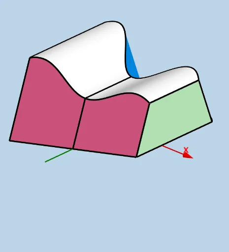
This example demonstrates a solid whose cross sections parallel to the y-axis are isosceles trapezoids, with the longer base equal to the difference between the upper and lower functions. It illustrates the calculus technique of finding volume by integrating cross-sectional areas. The construction uses GeoGebra commands such as Line, Rotate, Ray, Intersect, Circle, Segment, Translate, Midpoint, Sphere, Textfield, Polygon, Angle, CurveCartesian, Surface, and Mirror to build the dynamic solid. Users can adjust parameters like the upper/lower functions, rotation angle, and height via sliders and text fields, observing how the trapezoidal cross sections change. This is suitable for high school or college students studying integral calculus, solid geometry, and function graphing.
GeoGebra Commands & Parameters
Line(I, I + (1, 0, 0)) → f_1Rotate(H, (ANG * pi / 180), I, f_1) → H'Rotate(I, ((-ANG) * pi / 180), H, Plane[H', I, H]) → I'_1Ray(H, I'_1) → p_2Ray(I, H') → q_2Intersect(q_2, p_2) → W_1Circle(W_1, (SLratio * Distance[W_1, I]), Plane[W_1, I, H]) → e_2Intersect(q_2, e_2) → B_2, C_2Intersect(p_2, e_2) → Z_1, A_2Line(K, K + (1, 0, 0)) → tRotate(J, (ANG * pi / 180), K, t) → J'_1Ray(K, J'_1) → k_2Rotate(K, ((-ANG) * pi / 180), J, Plane[J'_1, K, J]) → K'Ray(J, K') → j_2Intersect(k_2, j_2) → R_1Circle(R_1, (SLratio * Distance[R_1, K]), Plane[J'_1, K, J]) → d_2Intersect(j_2, d_2) → U_1, V_1Intersect(k_2, d_2) → S_1, T_1Intersect(lower, h, (0, -9)) → CLine(C, C + (1, 0, 0)) → cIntersect(upper, h, (0, 5)) → BSegment(C, B) → qIntersect(upper, q, (0, 5)) → GRotate(G, (ANG * pi / 180), C, c) → G'_1Rotate(C, (ANG * pi / 180), G, Plane[G, C, G'_1]) → C'Ray(G, C') → f_2Ray(C, G'_1) → g_2Intersect(g_2, f_2) → M_1Circle(M_1, (SLratio * Distance[M_1, C]), Plane[C, G'_1, G]) → c_2Intersect(g_2, c_2) → N_1, O_1Intersect(f_2, c_2) → P_1, Q_1Translate(G'_1, Vector[C, G]) → J_1Segment(H, I) → s_1Midpoint(s_1) → A_1Segment(J, K) → q_1Midpoint(q_1) → ZMidpoint(s_1) → EMidpoint(q_1) → FMidpoint(C, G) → TLine(B, D) → iSphere(B, d) → eSegment(C, B) → pTextfield(upper) → InputBox1Textfield(lower) → InputBox2Textfield(a) → InputBox3Textfield(b) → InputBox4Segment(C, G) → k_1Line(C, G) → jSphere(G, T) → kLine(T, T + (1, 0, 0)) → mRotate(G, pi / 3, F_1, m) → G'Rotate(G', pi / 3, F_1, Line[F_1, F_1 + (1, 0, 0)]) → G''Line(F_1, F_1 + (1, 0, 0)) → nPolygon(C, G, Q_1, O_1) → poly1, g_1, m_1, r_1, a_1Rotate(G'', pi / 3, F_1, n) → G'''Rotate(G''', pi / 3, F_1, n) → G_1Line(Z, Z + (1, 0, 0)) → fLine(D_1, D_1 + (1, 0, 0)) → gRotate(J, pi / 3, D_1, g) → J'Rotate(J', pi / 3, D_1, g) → J''Rotate(J'', pi / 3, D_1, g) → J'''Rotate(J''', pi / 3, D_1, g) → E_1Line(H_1, H_1 - (1, 0, 0)) → l_1Rotate(I, pi / 3, H_1, l_1) → I'Rotate(I', pi / 3, H_1, l_1) → I''Rotate(I'', pi / 3, H_1, l_1) → I'''Rotate(I''', pi / 3, H_1, l_1) → I_1Translate(J'_1, Vector[K, J]) → K_1Polygon(K, J, V_1, T_1) → q1, j_1, l_2, m_2, n_2Polygon(I, H, A_2, C_2) → q2, e_1, h_2, i_2, f_3Translate(H', Vector[I, H]) → H''Intersect(t, q_1) → L_1Angle(G, C, G'_1) → αSegment(O_1, Q_1) → rSegment(G, Q_1) → lAngle(Q_1, G, C) → βSegment(O_1, C) → sSegment(T_1, L_1) → d_1Segment(J, V_1) → b_1Segment(T_1, V_1) → c_1Segment(C_2, I) → p_1Segment(H, A_2) → i_1Segment(A_2, C_2) → n_1CurveCartesian(t, (0.5 * (upper(t) + lower(t))) - ((SLratio * 0.5) * (upper(t) - lower(t))), ((((1 - SLratio) * 0.5) * (upper(t) - lower(t))) * tan((ANG * pi / 180))), t, a, b) → oCurveCartesian(t, (0.5 * (upper(t) + lower(t))) + ((SLratio * 0.5) * (upper(t) - lower(t))), ((((1 - SLratio) * 0.5) * (upper(t) - lower(t))) * tan((ANG * pi / 180))), t, a, b) → uSurface(u, lower(u) + ((((1 - SLratio) * 0.5) * (upper(u) - lower(u))) * v), (((((1 - SLratio) * 0.5) * (upper(u) - lower(u))) * tan((ANG * pi / 180))) * v), u, a, b, v, 0, 1) → o_1Surface(u, upper(u) - ((((1 - SLratio) * 0.5) * (upper(u) - lower(u))) * v), (((((1 - SLratio) * 0.5) * (upper(u) - lower(u))) * tan((ANG * pi / 180))) * v), u, a, b, v, 0, 1) → u_1Surface(u, lower(u) + (((1 - SLratio) * 0.5) * (upper(u) - lower(u))) + ((SLratio * (upper(u) - lower(u))) * v), ((((1 - SLratio) * 0.5) * (upper(u) - lower(u))) * tan((ANG * pi / 180))), u, a, b, v, 0, 1) → v_1Mirror(o_1, Plane[(0, 0, 0), (1, 0, 0), (1, 1, 0)]) → w_1Mirror(o, Plane[(0, 0, 0), (1, 0, 0), (1, 1, 0)]) → o'Mirror(u_1, Plane[(0, 0, 0), (1, 0, 0), (1, 1, 0)]) → a_2Mirror(v_1, Plane[(0, 0, 0), (1, 0, 0), (1, 1, 0)]) → b_2Mirror(J, Plane[(0, 0, 0), (1, 0, 0), (1, 1, 0)]) → J'_2Mirror(V_1, Plane[(0, 0, 0), (1, 0, 0), (1, 1, 0)]) → D_2Segment(J'_2, D_2) → r_2Mirror(T_1, Plane[(0, 0, 0), (1, 0, 0), (1, 1, 0)]) → E_2Mirror(L_1, Plane[(0, 0, 0), (1, 0, 0), (1, 1, 0)]) → F_2Segment(E_2, F_2) → s_2Mirror(T_1, Plane[(0, 0, 0), (1, 0, 0), (1, 1, 0)]) → G_2Mirror(V_1, Plane[(0, 0, 0), (1, 0, 0), (1, 1, 0)]) → H_2Segment(G_2, H_2) → t_2Mirror(poly1, Plane[(0, 0, 0), (1, 0, 0), (1, 1, 0)]) → poly1'Mirror(O_1, Plane[(0, 0, 0), (1, 0, 0), (1, 1, 0)]) → I_2Mirror(C, Plane[(0, 0, 0), (1, 0, 0), (1, 1, 0)]) → C'_1Segment(I_2, C'_1) → s'Mirror(O_1, Plane[(0, 0, 0), (1, 0, 0), (1, 1, 0)]) → J_2Mirror(Q_1, Plane[(0, 0, 0), (1, 0, 0), (1, 1, 0)]) → K_2Segment(J_2, K_2) → r'Mirror(G, Plane[(0, 0, 0), (1, 0, 0), (1, 1, 0)]) → G'_2Mirror(Q_1, Plane[(0, 0, 0), (1, 0, 0), (1, 1, 0)]) → L_2Segment(G'_2, L_2) → l'Mirror(u, Plane[(0, 0, 0), (1, 0, 0), (1, 1, 0)]) → u'Mirror(q1, Plane[(0, 0, 0), (1, 0, 0), (1, 1, 0)]) → q1'Mirror(q2, Plane[(0, 0, 0), (1, 0, 0), (1, 1, 0)]) → q2'Mirror(C_2, Plane[(0, 0, 0), (1, 0, 0), (1, 1, 0)]) → M_2Mirror(I, Plane[(0, 0, 0), (1, 0, 0), (1, 1, 0)]) → I'_2Segment(M_2, I'_2) → g_3Mirror(H, Plane[(0, 0, 0), (1, 0, 0), (1, 1, 0)]) → H'_1Mirror(A_2, Plane[(0, 0, 0), (1, 0, 0), (1, 1, 0)]) → N_2Segment(H'_1, N_2) → h_3Mirror(A_2, Plane[(0, 0, 0), (1, 0, 0), (1, 1, 0)]) → O_2Mirror(C_2, Plane[(0, 0, 0), (1, 0, 0), (1, 1, 0)]) → P_2Segment(O_2, P_2) → i_3Angle(J_2, C, G) → γAngle(L_2, G, C) → δTextfield(SLratio) → InputBox5
AI Drawing Prompt Reference
Create a 3D solid whose cross-sections parallel to the y-axis are isosceles trapezoids. The solid is bounded by upper and lower function curves, with the longer base of each trapezoid equal to the difference between the two functions. Use sliders to adjust the upper/lower functions, rotation angle, and height, observing how the trapezoidal sections change. The figure includes two main cross-sectional regions, each formed by two rays and an arc, creating symmetric trapezoidal outlines. The solid's surface is composed of multiple planes and curved patches, with key points, segments, and angle markers displayed. This dynamic geometry illustrates the calculus technique of volume by cross-sectional areas.
The prompt above was compiled from the original drawing commands and is for reference only.