Illustration of Volume as a Set of Nested Cylinders (Copy)

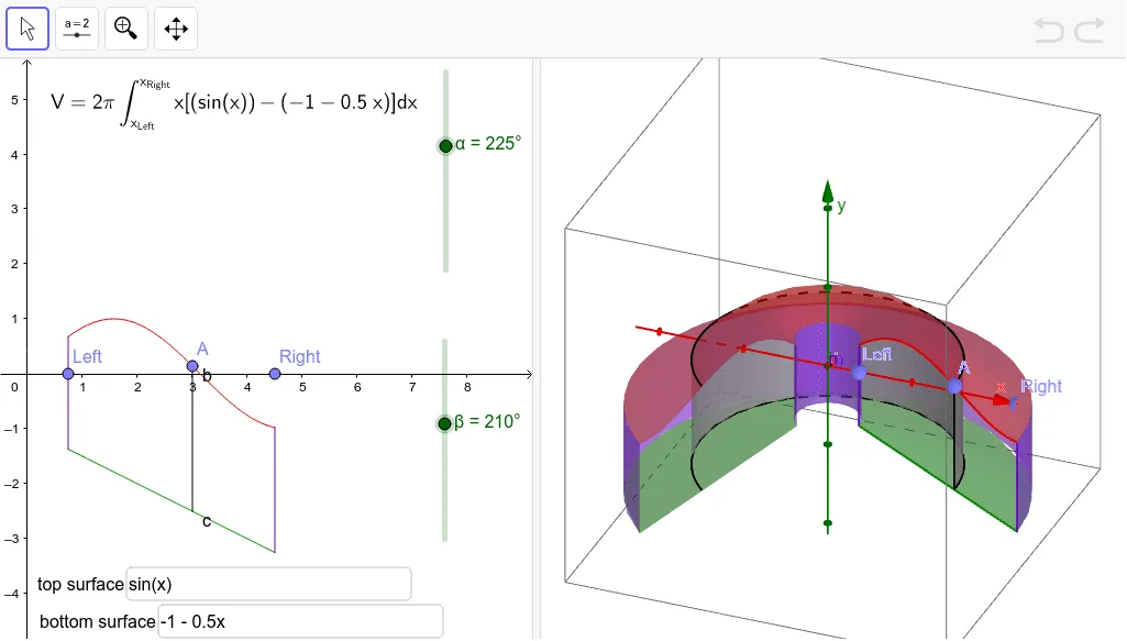
① This example visually demonstrates how the volume of a solid of revolution can be approximated by a set of nested cylindrical shells (or disks), showing the process of stacking thin cylinders to approach the true volume. ② Core mathematical concepts include the geometric meaning of definite integrals, the method of cylindrical shells/disks for computing volumes of revolution, and the limit concept underlying volume calculation. ③ Construction highlights: Using GeoGebra commands such as Point, Segment, Textfield, Surface, If, CurveCartesian, and LaTeX, the construction includes parameters for height (h), radius function (g), left/right boundaries (Left/Right), rotation axis (k), function f, points A and B, angles α and β, input boxes (inputBox1, inputBox2), sliders (j, l), and auxiliary objects (d, e, i, m, n, b, c) plus text1, allowing dynamic adjustment of the number and size of cylinders to visualize convergence. ④ Suitable for senior high school or introductory college calculus students, this interactive tool helps learners grasp the relationship between definite integrals and volume, and serves as an effective teaching aid for instructors explaining solids of revolution.