Volume of Revolution - Disks (W 3.1)

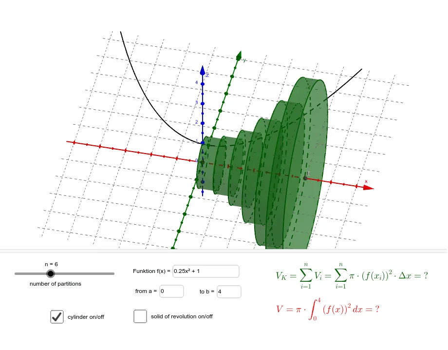
① This GeoGebra example dynamically demonstrates the calculation of the volume of a solid of revolution obtained by rotating a function curve around the x-axis using the disk method, visualizing how integral summation approximates the exact volume. ② Core mathematical concepts include definite integrals, volumes of revolution, infinitesimal disk elements, Riemann sum approximation, along with connections to the unit circle, Pythagorean theorem, and piecewise functions. ③ Construction highlights: the Sequence command generates partition points, Surface creates the revolved surface, Textfield provides interactive input boxes, a slider n controls the number of disks, and dynamic text objects display Δx, approximate volume V_K, and exact volume V. ④ Suitable for high school to early college calculus courses, particularly for teaching the geometric interpretation of definite integrals in volume computation and exploring how the number of subdivisions affects approximation accuracy.