
Comparing Numerical Integration Techniques
Loading the math board and drawing, please wait…
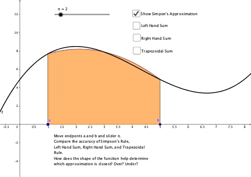
This example demonstrates different numerical integration methods, including upper sum, lower sum, rectangle sum, and trapezoidal sum. Students can intuitively understand the concept of integration and its applications through these methods. Core mathematical concepts include integration, rectangle sum, and trapezoidal sum. GeoGebra commands used include Point, Sequence, BarChart, Integral, LeftSum, RectangleSum, and TrapezoidalSum. Suitable for high school mathematics, particularly calculus courses.
GeoGebra Commands & Parameters
Point(xAxis) → APoint(xAxis) → BSequence(a + (i * Δx), i, 0, n) → XSequence(Element[X, i] + Δx / 2, i, 1, n) → X2Sequence(a + (i * Δx) + (Δx * random()), i, 0, n - 1) → RandListBarChart(a, b, f(RandList)) → RandApproxSequence(Determinant[{{Element[X, (2 * i) - 1], f(Element[X, (2 * i) - 1]), 1}, {Element[X, (2 * i)], f(Element[X, (2 * i)]), 1}, {Element[X, (2 * i) + 1], f(Element[X, (2 * i) + 1]), 1}}], i, 1, n / 2, 1) → PSequence(Determinant[{{Element[X, (2 * i) - 1]^(2), f(Element[X, (2 * i) - 1]), 1}, {Element[X, (2 * i)]^(2), f(Element[X, (2 * i)]), 1}, {Element[X, (2 * i) + 1]^(2), f(Element[X, (2 * i) + 1]), 1}}], i, 1, n / 2, 1) → QSequence(Determinant[{{Element[X, (2 * i) - 1]^(2), Element[X, (2 * i) - 1], f(Element[X, (2 * i) - 1])}, {Element[X, (2 * i)]^(2), Element[X, (2 * i)], f(Element[X, (2 * i)])}, {Element[X, (2 * i) + 1]^(2), Element[X, (2 * i) + 1], f(Element[X, (2 * i) + 1])}}], i, 1, n / 2, 1) → RSequence(Determinant[{{Element[X, (2 * i) - 1]^(2), Element[X, (2 * i) - 1], 1}, {Element[X, (2 * i)]^(2), Element[X, (2 * i)], 1}, {Element[X, (2 * i) + 1]^(2), Element[X, (2 * i) + 1], 1}}], i, 1, n / 2, 1) → SSequence(If[x ≥ Element[X, (2 * i) - 1] ∧ x ≤ Element[X, (2 * i) + 1], (-1 / Element[S, i] * ((Element[P, i] * x^(2)) - (Element[Q, i] * x) - Element[R, i]))], i, 1, n / 2) → simpSequence((Element[X, i], f(Element[X, i])), i, 1, n + 1) → pointsIntegral(Element[simp, 1], Element[X, 1], Element[X, 3]) → dIntegral(Element[simp, 2], Element[X, 3], Element[X, 5]) → gIntegral(Element[simp, 3], Element[X, 5], Element[X, 7]) → hIntegral(Element[simp, 4], Element[X, 7], Element[X, 9]) → jIntegral(Element[simp, 5], Element[X, 9], Element[X, 11]) → kIntegral(Element[simp, 6], Element[X, 11], Element[X, 13]) → lIntegral(Element[simp, 7], Element[X, 13], Element[X, 15]) → oIntegral(Element[simp, 8], Element[X, 15], Element[X, 17]) → pIntegral(Element[simp, 9], Element[X, 17], Element[X, 19]) → qIntegral(Element[simp, 10], Element[X, 19], Element[X, 21]) → rLeftSum(f, a, b, n) → vRectangleSum(f, a, b, n, 1) → wTrapezoidalSum(f, a, b, n) → a_1Segment(A, C) → f_1Segment(B, D) → g_1
AI Drawing Prompt Reference
Draw a coordinate plane with a function curve. Mark two points on the x-axis as the integration interval endpoints, and divide the interval into equal subintervals. Visualize different numerical integration methods: use random-height bars for random sampling, left-endpoint rectangles, midpoint rectangles, and trapezoids. Also fit quadratic polynomials to consecutive sample points and shade the areas under these parabolas. Connect the interval endpoints to the curve with line segments to compare approximation accuracy.
The prompt above was compiled from the original drawing commands and is for reference only.