
Mixed Coordinate System: Natural Space-time Geometry
Loading the math board and drawing, please wait…
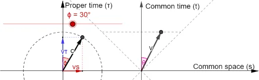
This example visualizes the geometric relationship between natural space-time (proper time plus common space) and common space-time within a mixed coordinate system. Key concepts include coordinate transformations, vectors, and angles. Construction utilizes GeoGebra commands such as Circle, Vector, Segment, Angle, and Text to define objects like O, C, P, and variables ϕ, σ. Suitable for high school or university students studying mathematical physics or geometry to understand coordinate system transformations.
GeoGebra Commands & Parameters
Circle(O, 1) → CVector(O, P) → σVector(O, pτ) → vτVector(O, ps) → vsSegment(P, ps) → ssSegment(P, pτ) → sτAngle(σ, Vector[O, (0, 1)]) → aϕSegment(Oa + (-1, 1), Oa + (1, 1)) → svjVector(Oa, Pa) → vAngle(v, Vector[Oa, Oa + (0, 1)]) → aθText(RotateText["s = c{\cdot}t", 45°], Oa + (0.25, 1), true, true) → txtctText(RotateText["s = -c{\cdot}t", (-(45°))], Oa + (-1, 1), true, true) → txtctcVector((x(Oa), -3), (x(Oa), 1.8)) → tiText("Common time (t)", Oa + (0.1, 1.6)) → txttil