
Lawson Minimal Surface on a Klein Bottle via 3D Projections
Loading the math board and drawing, please wait…
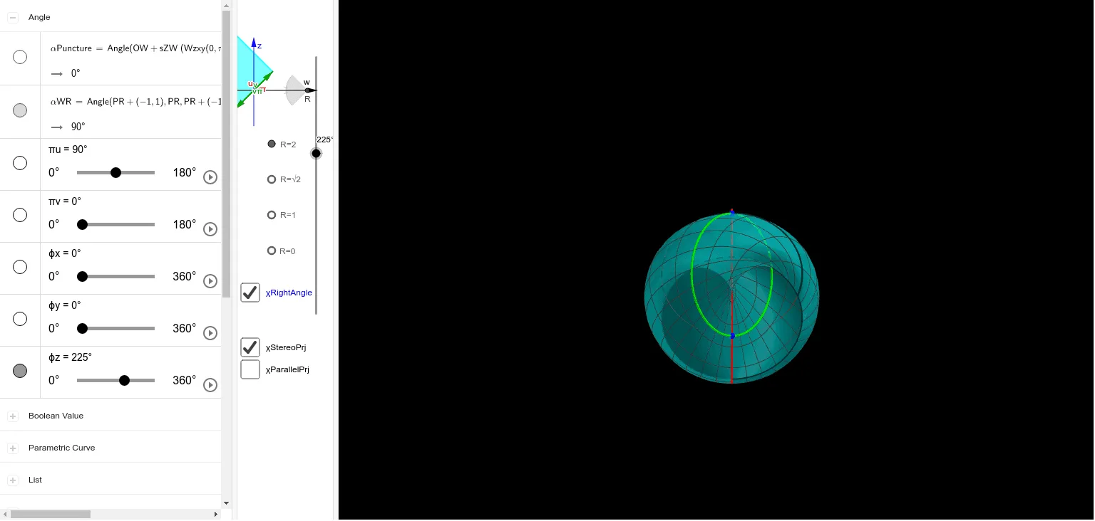
This example demonstrates how the Lawson minimal surface on a Klein bottle can be visualized by constructing a parameterized 3D surface and mapping it through geometric projection tools. It centers on key ideas from geometry and calculus-related visualization: minimal surfaces (the visual/structural hallmark of extremal/zero-mean-curvature behavior), the Klein bottle as a non-orientable surface, parameterized curve/surface modeling, and the use of parallel and stereo (stereographic-style) projections to render the geometry in 3D. Construction-wise, it leverages commands such as If, Text, Vector, Polygon, Angle, Sequence, Surface, and CurveCartesian to define parameter variables, direction vectors, angle constraints, and generate both the surface and supporting curves. Sequence is used for parameter sampling, Vector and Angle fix orientations, while Surface and CurveCartesian create the mesh-like minimal surface and related boundary/guide curves. Projection objects (e.g., ParallelPrjRays, StereoPrj, and derived projection variables) translate the parameter-domain construction into view-space, with Polygon and intermediate point/vector constructions coordinating the local geometry. Suitable for advanced high school and undergraduate audiences in solid/space geometry, parametric modeling, and early differential-geometry visualization.
GeoGebra Commands & Parameters
If(χStereoPrj, StereoPrj(x, y), If[χParallelPrj, (x * 6), 0]) → PrjText("x^2+z^2=y^2+w^2=1 ↔ x^2+w^2=y^2+z^2=1; Rotate: ϕ=arg(z,w); Stereo-projected from w=R", (0, 0), false, true) → txtExplainVector(OW - (1, 0), OW + (1.8, 0)) → vWPolygon(OW + (sZW * (Wzxy(0, 0), Zw(0, 0))), OW + (sZW * (Wzxy(0, π), Zw(0, π))), 4) → TZWVector(OW - (0, 1), OW + (0, 1.5)) → vZAngle(PR + (-1, 1), PR, PR + (-1, -1)) → αWRSequence(Vector[PR + (0, z), PR + (-0.1, z)], z, -1, 1, 0.1) → ParallelPrjRaysVector(OW + (sZW * (Wzxy(0, 0), Zw(0, 0))), OW + (sZW * (Wzxy(π, 0), Zw(π, 0)))) → vZWUVector(OW + (sZW * (Wzxy(0, π), Zw(0, π))), OW + (sZW * (Wzxy(π, π), Zw(π, π)))) → vZWUπVector(OW + (sZW * (Wzxy(0, 0), Zw(0, 0))), OW + (sZW * (Wzxy(0, π), Zw(0, π)))) → vZWVVector(OW + (sZW * (Wzxy(π, 0), Zw(π, 0))), OW + (sZW * (Wzxy(π, π), Zw(π, π)))) → vZWVπAngle(OW + (sZW * (Wzxy(0, π), Zw(0, π))), OW + (sZW * (Wzxy(0, 0), Zw(0, 0))), OW + (sZW * (Wzxy(π, 0), Zw(π, 0)))) → αPunctureVector(PUV00, PUV00 + (0, 2, 0)) → vV00Vector(PUV0π, PUV0π + (0, -2, 0)) → vV0πVector(PUVπ0, PUVπ0 + (0, 2, 0)) → vVπ0Vector(PUVππ, PUVππ + (0, -2, 0)) → vVππVector(PUV0π, PUV0π + (2, 0, 0)) → vU0πVector(PUVπ0, PUVπ0 + (-2, 0, 0)) → vUπ0Vector(PUV00, PUV00 + (2, 0, 0)) → vU00Vector(PUVππ, PUVππ + (-2, 0, 0)) → vUππSurface(PrjX(u, v), PrjY(u, v), PrjZ(u, v), u, 0, (2 * π), v, (-0.005 * π), (0.005 * π)) → ShellUCurveCartesian(PrjX(u, π), PrjY(u, π), PrjZ(u, π), u, 0, (2 * π)) → ShellUπCurveCartesian(PrjX(π, v), PrjY(π, v), PrjZ(π, v), v, 0, (2 * π)) → ShellVπSurface(PrjX(u, v), PrjY(u, v), PrjZ(u, v), u, (-0.005 * π), (0.005 * π), v, 0, (2 * π)) → ShellVSurface(PrjX(u, v), PrjY(u, v), PrjZ(u, v), u, πu, (2 * π) - πu, v, πv, (2 * π) - πv) → ShellCurveCartesian(PrjX(u, πv), PrjY(u, πv), PrjZ(u, πv), u, πu, (2 * π) - πu) → ShellEdgeUCurveCartesian(PrjX(u, (-πv)), PrjY(u, (-πv)), PrjZ(u, (-πv)), u, πu, (2 * π) - πu) → ShellEdgeUnCurveCartesian(PrjX(πu, v), PrjY(πu, v), PrjZ(πu, v), v, πv, (2 * π) - πv) → ShellEdgeVCurveCartesian(PrjX((-πu), v), PrjY((-πu), v), PrjZ((-πu), v), v, πv, (2 * π) - πv) → ShellEdgeVn
AI Drawing Prompt Reference
Draw a visualization of the Lawson minimal surface on a Klein bottle. The figure should include a parameterized minimal surface model rendered via parallel and stereographic projections. Key objects are the surface itself, auxiliary curves (boundary and guide curves), direction vectors, and angle constraints. The construction order is: first define parameter variables and direction vectors, then build the surface and related curves, followed by applying projection tools to map the parameter domain to view space, and finally coordinating local geometry to present the complete figure. The figure should reflect the non-orientable surface and minimal curvature characteristics, suitable for geometric modeling and visualization education.
The prompt above was compiled from the original drawing commands and is for reference only.