
Mean Value and Rolle's Theorems Visualization
Loading the math board and drawing, please wait…
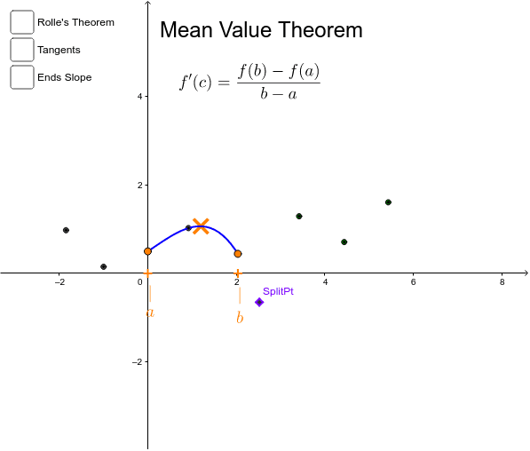
This example visually demonstrates the Mean Value Theorem and Rolle's Theorem, highlighting key points marked with X to illustrate the core concepts of the theorems. It involves fundamental calculus ideas such as derivatives, continuity, extrema, and geometric interpretations. The construction utilizes GeoGebra commands like Sort, Take, Polynomial, Point, Max, Min, Element, Line, Tangent, and Zip, along with objects like points, lines, and tangents, to plot functions and mark critical locations. Suitable for high school and above students learning calculus, this tool aids in understanding the application of these fundamental theorems.
GeoGebra Commands & Parameters
Sort({A, B, C, D, E, F, G}) → slistTake(slist, 4) → lrightPolynomial(lright) → prightTake(slist, 1, 4) → lleftPolynomial(lleft) → pleftPoint(xAxis) → HPoint(xAxis) → IMax(xH, xI) → xRightMin(xH, xI) → xLeftElement(slist, 4) → SplitPtSort({Extremum[rol, xLeft, xRight]}) → lextLine(Hend, Iend) → aTangent(Element[lext, 1], rol) → RTan1Tangent(Element[lext, 2], rol) → RTan2Tangent(Element[lext, 3], rol) → RTan3Tangent(Element[lext, 4], rol) → RTan4Tangent(Element[xext, 1], psplit) → MTan1Tangent(Element[xext, 2], psplit) → MTan2Tangent(Element[xext, 3], psplit) → MTan3Tangent(Element[xext, 4], psplit) → MTan4Line(Mleft, Mright) → cZip((xVal, psplit(xVal)), xVal, xext) → pext