
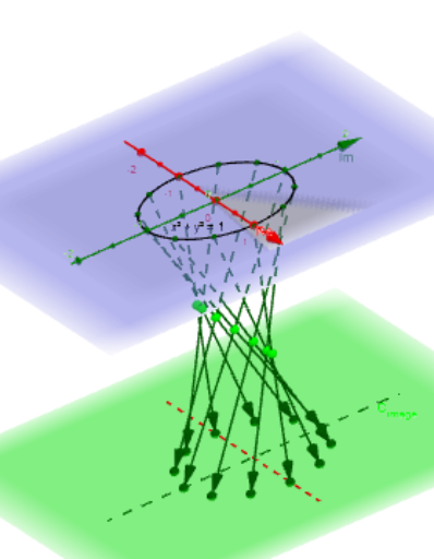
Mapping Diagram of Powers Homotopy
Loading the math board and drawing, please wait…
In collections
Mapping Diagrams to Visualize Complex Analysis
This example demonstrates the homotopy mapping diagram of power functions with varying parameters. Key mathematical concepts include power functions, homotopy transformations, and mapping diagrams. Using GeoGebra commands like Sequence, Vector, and Textfield, the dynamic changes in the power function graphs can be shown. Suitable for high school mathematics education and learning, particularly in coordinate geometry and function transformations.
GeoGebra Commands & Parameters
Sequence(t, t, t_0, t_2, dt) → t_*Zip((r * ℯ^((B * ί))), B, t_*) → z_*Zip((x(B), y(B), hi), B, fz_*) → fpoint_*Vector(z_#, f_{(z#).}) → wTextfield(f_{(z#)}) → inputBox2CurveCartesian(t, 0, hi, t, -5, 5) → XhCurveCartesian(0, t, hi, t, -5, 5) → YhTextfield(z_*) → inputBox3Zip(Vector[A, B], A, z_*, B, fpoint_*) → fvec_*Zip(Line[A, B], A, z_*, B, fpoint_*) → list1Zip(Intersect[h, Line[A, B]], A, z_*, B, fpoint_*) → Homotpts
AI Drawing Prompt Reference
Create a dynamic homotopy mapping diagram for power functions, showing continuous deformation of function graphs as parameters change. Draw two coordinate axes, generate a series of power function graphs based on parameters, and connect corresponding points with vectors to illustrate the mapping relationship. Label key points and parameters, and use text boxes to display the dynamic function expressions and parameter values, presenting the geometric intuition of function transformations.
The prompt above was compiled from the original drawing commands and is for reference only.