
Mapping Diagram for z^n with Curve on Riemann Surface
Loading the math board and drawing, please wait…
In collections
Mapping Diagrams to Visualize Complex Analysis
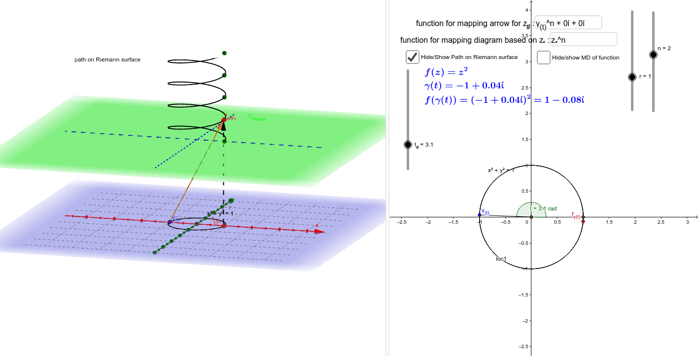
This example demonstrates the mapping diagram for the complex power function z^n, with a visualization of the image curve on the Riemann surface. Key math concepts include complex numbers, mapping, Riemann surfaces, and parametric equations. Construction highlights involve GeoGebra commands like Sequence, CurveCartesian, Textfield, Vector, Locus, Intersect, Segment, and Angle, along with objects such as t_#, r, e, z_*, n, b, a, height_{image}, C_{image}, fz_*, C_{domain}, γ_{(t)}, f_{γ(t)}, f_{(z#).}, fpoint_*, fvec_*, d, inputBox1, w, inputBox2, Xh, Yh, inputBox3, c, text2, loc1, text3, A, δ, B, t, u, f, text4, text5, text6, text7, text8, wndg_{#}, text1. Suitable for high school and above students to understand the geometric meaning of complex functions and the construction of Riemann surfaces.
GeoGebra Commands & Parameters
Sequence((r * (cos(t) + (sin(t) * ί))), t, -3.141592653589793, 3.141592653589793, 0.5235987755982988) → z_*Sequence((x(Element[fz_*, k]), y(Element[fz_*, k]), height_{image}), k, 1, 12) → fpoint_*Sequence(Vector[Element[z_*, j], Element[fpoint_*, j]], j, 1, 12) → fvec_*CurveCartesian((r * cos(t)), (r * sin(t)), height_{image}, t, 0, 6.283185307179586) → dTextfield(fz_*) → inputBox1Vector(γ_{(t)}, f_{(z#).}) → wTextfield(f_{γ(t)}) → inputBox2CurveCartesian(t, 0, height_{image}, t, -5, 5) → XhCurveCartesian(0, t, height_{image}, t, -5, 5) → YhTextfield(z_*) → inputBox3Locus(f_{(z#).}, t_#) → loc1Intersect(xAxis, yAxis) → ASegment(γ_{(t)}, A) → δIntersect(c, xAxis, 2) → BAngle(B, A, γ_{(t)}) → tVector(f_{γ(t)}, f_{(z#).}) → uSequence((1, 0, t / 4 + 3), t, 0, (4 * π), (2 * π / n)) → wndg_{#}