Mapping Diagram for Möbius Transformation: Roots and Poles, Lines and Circles

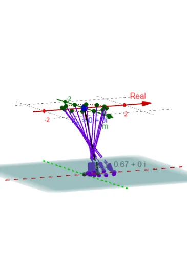
This GeoGebra example demonstrates the mapping diagram of a Möbius transformation (fractional linear transformation), showing how lines and circles in the complex plane are mapped to lines or circles, with roots and poles highlighted. Core mathematical concepts include Möbius transformations, conformal mapping, preservation of generalized circles, roots and poles, and complex plane geometry. The construction uses commands such as Sequence, Zip, Line, Circle, If, Vector, and Textfield to create dynamic objects including the transformation function f, grid lines, circles, vector fields, root/pole markers, and interactive input boxes and sliders. Suitable for university complex analysis courses or advanced high school math, this example helps visualize the geometric properties and mapping behavior of fractional linear transformations.