Mapping Diagram for Complex Power Function (Circles)

Loading the math board and drawing, please wait…

2015-02-02 07:08

In collections Mapping Diagrams to Visualize Complex Analysis

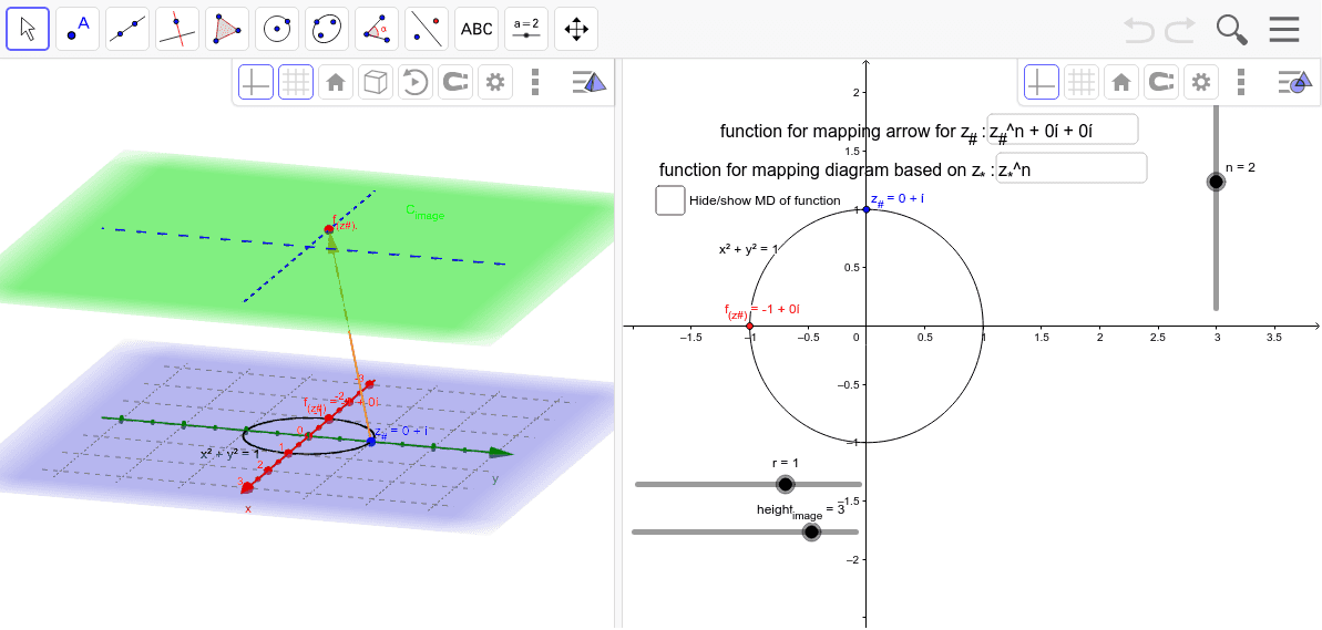
This example visualizes complex power functions using a mapping diagram, focusing on circular representations. It involves core concepts like complex numbers, power functions, mapping relations, and coordinate geometry. The construction utilizes GeoGebra commands such as Sequence, Point, CurveCartesian, Textfield, and Vector to create the visualization. Suitable for high school and above, it helps in understanding the geometric interpretation and transformations of complex functions.

GeoGebra Commands & Parameters

Sequence((r * (cos(t) + (sin(t) * ί))), t, -3.141592653589793, 3.141592653589793, 0.5235987755982988) → z_*
Point(c) → z_#
Sequence((x(Element[fz_*, k]), y(Element[fz_*, k]), height_{image}), k, 1, 12) → fpoint_*
Sequence(Vector[Element[z_*, j], Element[fpoint_*, j]], j, 1, 12) → fvec_*
CurveCartesian((r * cos(t)), (r * sin(t)), height_{image}, t, 0, 6.283185307179586) → d
Textfield(fz_*) → inputBox1
Vector(z_#, f_{(z#).}) → w
Textfield(f_{(z#)}) → inputBox2
CurveCartesian(t, 0, height_{image}, t, -5, 5) → Xh
CurveCartesian(0, t, height_{image}, t, -5, 5) → Yh
Textfield(z_*) → inputBox3