Mapping Diagram for Complex Integration over a Circle

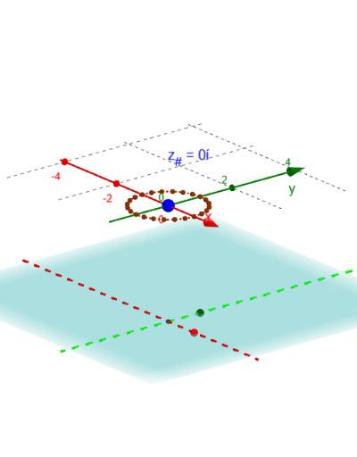
This GeoGebra example dynamically illustrates the mapping diagram for a complex integral along a circular path. It visualizes how points on the integration contour (a circle) are mapped by a complex function to the image plane, using vector fields and locus traces to show the Riemann-sum approximation of the integral. Core mathematical concepts include complex integration, parametrized curves, complex mappings, vector fields, and discretization of the integration path. Construction highlights: Sequence generates discrete sample points, Circle defines the contour, Line and Vector draw mapping arrows, Locus traces the image points, ToComplex converts coordinates to complex numbers, and Textfield/InputBox allow interactive input of the function and parameters. This is suitable for university-level complex analysis courses or advanced undergraduates, and serves as a powerful teaching tool for instructors to demonstrate the geometric meaning and numerical approximation of complex line integrals.