
Mapping Diagram Composition Adjust Arrows
Loading the math board and drawing, please wait…
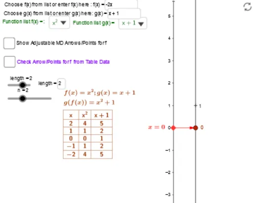
This example demonstrates the composition of mapping diagrams and allows users to adjust arrows. Key mathematical concepts include functions and vectors. Using GeoGebra commands such as Point, Vector, and Sequence, users can visually understand the geometric meaning of function composition. Suitable for high school mathematics education and learning.
GeoGebra Commands & Parameters
Point(y_{axis}) → P5Point(y_{axis}) → P9Point(y_{axis}) → P8Point(y_{axis}) → P7Point(y_{axis}) → P6Point(y_{axis}) → P4Point(y_{axis}) → P3Point(y_{axis}) → P2Point(y_{axis}) → P1SelectedElement(flist) → fPoint(yAxis) → AIf(d ≟ 1, y(A) - f(y(A)), 0) → alignVector(A, B) → uTextfield(f) → inputBox1Textfield(length) → inputBox4Sequence(t, t, y(A) + (n * Δx), y(A) - (n * Δx), (-Δx)) → t_*Zip((k, f(k)), k, t_*) → GraphfptsZip((0, k), k, t_*) → SourcePtsMDZip(f(k), k, t_*) → ft_*Zip((2, (y_{zoom} * (k + align))), k, ft_*) → fTargPtsZip(Vector[(0, k), (2, (y_{zoom} * (m + align)))], k, t_*, m, ft_*) → farrVector(X_1, Y_1) → vLine(A, B) → hIntersect(f1, h, (2.7851193573624755E-10, -5.570238714724951E-10)) → CZip(Vector[A, B], A, SourcePtsMD, B, fTGTpts) → fTGTarrTextfield(f1) → inputBox2SelectedElement(glist) → gPoint(i) → Q5Point(i) → Q1Point(i) → Q2Point(i) → Q3Point(i) → Q4Point(i) → Q6Point(i) → Q7Point(i) → Q8Point(i) → Q9Zip((4, A), A, gft_*) → gTargPtsZip(Vector[A, B], A, fTargPts, B, gTargPts) → garrTableText(Transpose[{Join[{{"x"}, t_*}], Join[{{f}, ft_*}], Join[{{g}, gft_*}]}], "|_cc") → text13Zip(Vector[A, B], A, fTargPts, B, gTGTpts) → gTGTarrTextfield(g1) → InputBox1Zip((A, g(f(A))), A, t_*) → Graphgfpts
AI Drawing Prompt Reference
Draw a mapping diagram for function composition, showing arrows from a vertical axis on the left through a middle axis to a right axis. Place sample points on the left axis, connect them horizontally to the middle axis representing f(x), then draw arrows to the right axis for g(f(x)). Include editable text boxes for function inputs and draggable points to adjust arrow positions. Display a table with columns for x, f(x), and g(f(x)), and plot points of the composed function. The layout has three vertical axes with arrows flowing left-to-middle-to-right, illustrating the composition process.
The prompt above was compiled from the original drawing commands and is for reference only.