
Mapping Diagram: Complex Integration of 1/z
Loading the math board and drawing, please wait…
In collections
Mapping Diagrams to Visualize Complex Analysis
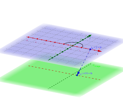
This example demonstrates the mapping diagram of the complex function 1/z, illustrating its geometric transformation and integration in the complex plane. Key math concepts include complex integration, mapping, and geometric transformations. GeoGebra commands like Sequence, Zip, Vector, CurveCartesian, Sphere, Intersect, Segment, and Textfield are used in its construction. Suitable for high school and above students to understand the geometric meaning of complex functions and the integration process.
GeoGebra Commands & Parameters
Sequence(t, t, t_0 + dt, t_1 + dt, dt) → t_3Zip(x_C(B) + (y_C(B) * ί), B, t_3) → z_1Sequence(t, t, t_0, t_1, dt) → t_*Zip(x_C(B) + (y_C(B) * ί), B, t_*) → z_*Zip(t - u, t, z_1, u, z_*) → dz_*Sequence((Element[fz_*, k] * Element[dz_*, k]), k, 1, n) → fdz_*Sequence(Sum[fdz_*, k], k, 1, n) → SUMfdz_*Zip((x(B), y(B), ht), B, fz_*) → fpoint_*Vector(z_#, f_{(z#).}) → wCurveCartesian(t, 0, ht, t, -5, 5) → XhCurveCartesian(0, t, ht, t, -5, 5) → YhSphere((0, 0, 4), 1) → RSIntersect(zAxis, RS, 2) → ASegment(A, f_{(z#).}) → f_sIntersect(f_s, RS) → P_∞, CZip((x(Z), y(Z), ht), Z, SUMfdz_*) → ESumSequence(Element[dz_*, k], k, 1, n) → dz_nCurveCartesian(x_C(t), y_C(t), t, t_0, t_1) → cTextfield(x_C) → inputBox4Textfield(y_C) → inputBox5Vector(z_#, Pointfz_#) → uTextfield(F) → InputBox1Zip(Vector[A, B], A, z_*, B, ESum) → ESumV_*Zip(Vector[A, B], A, z_*, B, fpoint_*) → fvec_*
AI Drawing Prompt Reference
Draw a 3D coordinate system illustrating the mapping and integration of the complex function 1/z. On the horizontal complex plane, show a curve as the integration path, with a series of points along it. From each point, draw a vertical vector to its mapped function value point at a fixed height, forming a mapped curve. Place a sphere above, centered on the vertical axis, and draw segments from path points to their mapped points, intersecting the sphere to create a trajectory on its surface. Use arrow vectors to represent small increments and cumulative sums. Include input boxes for adjusting path parameters and the function expression, showing the geometric transformation and integration process.
The prompt above was compiled from the original drawing commands and is for reference only.