Mapping Diagram and Graph for Estimating Derivatives

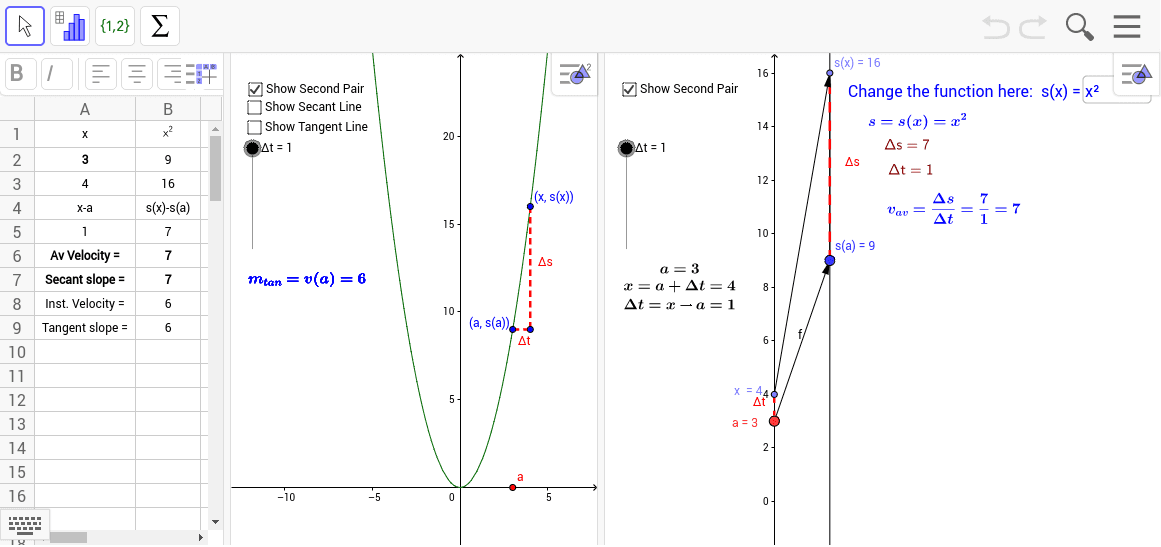
This example illustrates how to estimate the derivative of a function using a graph and a mapping diagram. It demonstrates the concept of derivatives, function graphs, normal distribution, complex numbers, random variables, rectangles, and calculus. The construction involves GeoGebra commands like Point, Vector, Textfield, Segment, Line, Intersect, Derivative, and objects such as Δt, a, A, f_1, B, f, inputBox1, x_0, f_x, G1, H1, A1, I1, J1, button1, x_1, y_1, v, E, F, c, d, e, g, Δs, j, i, k, Focus, l, inputBox2, text3, text4, secant, text1, b, text5, h, tangent, m. This is suitable for high school and above students learning calculus to understand the geometric meaning and calculation of derivatives.