
Lotka-Volterra Predator-Prey Model
Loading the math board and drawing, please wait…
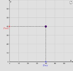
This example demonstrates the dynamic behavior and phase plane of the Lotka-Volterra predator-prey model. Key mathematical concepts include differential equations, population dynamics, oscillatory behavior, derivatives, and integrals. GeoGebra commands used in construction include SolveODE (solving differential equations), Length (calculating length), First (getting the first element of a list), Sequence (generating a sequence), Max (finding the maximum value), PolyLine (creating a polyline), Polygon (creating a polygon), Vector (creating a vector), Element (accessing an element), Textfield (creating a text field), and Segment (creating a segment). Suitable for high school students and learners interested in population dynamics models.
GeoGebra Commands & Parameters
SolveODE(DY, DX, x(A), y(A), t, step) → solutiondeLength(solutionde) → pointsFirst(solutionde, points) → solutionpointsSequence(x(Element[solutionpoints, i]), i, 1, N) → list1Sequence(y(Element[solutionpoints, i]), i, 1, N) → list2Max(list1) → maximum1Max(list2) → maximum2Sequence(((2 * i / N), Element[list1, i] / maximum22 + 1.5), i, 1, N) → list3Sequence(((2 * i / N), Element[list2, i] / maximum22 + 1.5), i, 1, N) → list4PolyLine(list3) → PreyPolyLine(list4) → PredatorPolygon(C, D, F, E) → poly1, c_1, d_1, f, eVector(G, I) → uVector(G, H) → vElement(solutionpoints, N) → JTextfield(x_0) → InputBox1Textfield(y_0) → InputBox2Segment(K, J) → gSegment(L, J) → hSolveODE(DY, DX, x(A), y(A), tiempos - step, step) → sol02