
Long Run Probability Analysis
Loading the math board and drawing, please wait…
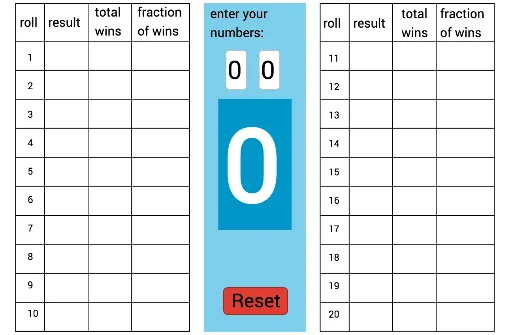
This example demonstrates the concept of long-run probability. It simulates multiple trials to show the stability of probability. Core math concepts include probability and statistics. The construction uses commands like Element, If, Length, Intersect, Point, Segment, Sequence, Textfield, Polygon in GeoGebra. Suitable for high school and above students learning probability and statistics.
GeoGebra Commands & Parameters
Element(recordk, 1) → u_1If(u_1 ≟ n_1 ∨ u_1 ≟ n_2, 1, 0) → w_1Element(recordk, 2) → u_2If(u_2 ≟ n_1 ∨ u_2 ≟ n_2, 1, 0) → w_2Element(recordk, 20) → u_{20}Element(recordk, 18) → u_{18}Element(recordk, 16) → u_{16}Element(recordk, 14) → u_{14}Element(recordk, 12) → u_{12}Element(recordk, 10) → u_{10}Element(recordk, 8) → u_8Element(recordk, 6) → u_6Element(recordk, 5) → u_5Element(recordk, 4) → u_4Element(recordk, 3) → u_3Element(recordk, 7) → u_7Element(recordk, 9) → u_9Element(recordk, 11) → u_{11}Element(recordk, 13) → u_{13}Element(recordk, 15) → u_{15}Element(recordk, 17) → u_{17}Element(recordk, 19) → u_{19}If(u_{20} ≟ n_1 ∨ u_{20} ≟ n_2, 1, 0) → w_{20}If(u_{18} ≟ n_1 ∨ u_{18} ≟ n_2, 1, 0) → w_{18}If(u_{16} ≟ n_1 ∨ u_{16} ≟ n_2, 1, 0) → w_{16}If(u_{14} ≟ n_1 ∨ u_{14} ≟ n_2, 1, 0) → w_{14}If(u_{12} ≟ n_1 ∨ u_{12} ≟ n_2, 1, 0) → w_{12}If(u_{10} ≟ n_1 ∨ u_{10} ≟ n_2, 1, 0) → w_{10}If(u_8 ≟ n_1 ∨ u_8 ≟ n_2, 1, 0) → w_8If(u_6 ≟ n_1 ∨ u_6 ≟ n_2, 1, 0) → w_6If(u_5 ≟ n_1 ∨ u_5 ≟ n_2, 1, 0) → w_5If(u_4 ≟ n_1 ∨ u_4 ≟ n_2, 1, 0) → w_4If(u_3 ≟ n_1 ∨ u_3 ≟ n_2, 1, 0) → w_3If(u_7 ≟ n_1 ∨ u_7 ≟ n_2, 1, 0) → w_7If(u_9 ≟ n_1 ∨ u_9 ≟ n_2, 1, 0) → w_9If(u_{11} ≟ n_1 ∨ u_{11} ≟ n_2, 1, 0) → w_{11}If(u_{13} ≟ n_1 ∨ u_{13} ≟ n_2, 1, 0) → w_{13}If(u_{15} ≟ n_1 ∨ u_{15} ≟ n_2, 1, 0) → w_{15}If(u_{17} ≟ n_1 ∨ u_{17} ≟ n_2, 1, 0) → w_{17}If(u_{19} ≟ n_1 ∨ u_{19} ≟ n_2, 1, 0) → w_{19}Length(recordk) → sIntersect(xAxis, yAxis) → APoint(xAxis) → BPoint(xAxis) → CPoint(xAxis) → DPoint(xAxis) → EPoint(yAxis) → FSegment(F, A) → fSegment(B, G) → gSegment(H, C) → hSegment(I, D) → iSegment(E, J) → jSegment(A, E) → kSegment(F, J) → lSequence(Segment[A + (0, i), E + (0, i)], i, 0, 10) → list1Sequence(Segment[K + (0, i), O + (0, i)], i, 0, 10) → list2Segment(P, K) → mSegment(L, G_1) → nSegment(M, H_1) → pSegment(I_1, N) → qSegment(O, J_1) → rSegment(J_1, P) → bTextfield(n_1) → InputBox11Textfield(n_2) → InputBox12Polygon(Q_1, Q_2, R, Q) → poly1, q_1, q_2, s_2, q_3Polygon(S, T, U, V) → poly2, s_1, t_1, u, v
AI Drawing Prompt Reference
Draw a coordinate system with points A, B, C, D, E on the x-axis and point F on the y-axis. Connect F and A to form line segment f. Simulate multiple trials and record the results u_1 to u_20. If u_i equals n_1 or n_2, mark it as 1; otherwise, mark it as 0, using w_i to represent these marks. Plot the distribution of these marks to observe the stability of long-run probability.
The prompt above was compiled from the original drawing commands and is for reference only.