
Logarithmic Spiral in Hexagonal Context
Loading the math board and drawing, please wait…
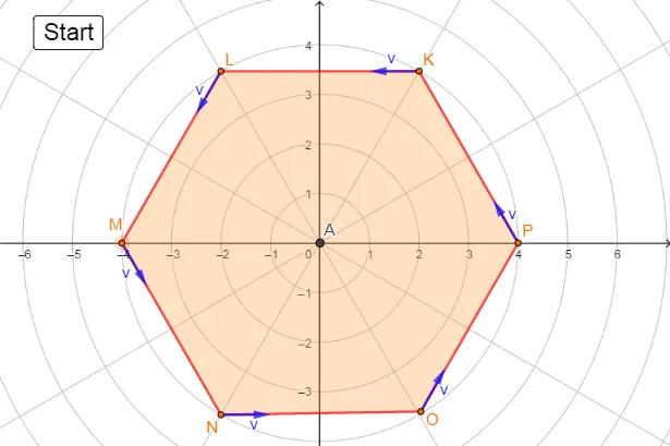
This GeoGebra example constructs a logarithmic spiral within a hexagonal framework, illustrating the interplay between logarithmic and exponential functions and geometric symmetry. Core concepts include logarithmic functions, exponential growth/decay, parametric curve representation, geometric transformations, tangents, and polygonal symmetry. Construction utilizes GeoGebra commands such as Intersect, Point, Segment, Circle, Length, CurveCartesian, Line, Mirror, LineBisector, Polygon, Tangent, and Vector, employing points, circles, polygons, and mirror transformations to generate the spiral trajectory. Ideal for high school and early university students studying function geometry, analytic geometry, or calculus introduction, it provides a visual and interactive means to explore parameterized curves and the geometric interpretation of logarithmic behavior.
GeoGebra Commands & Parameters
Intersect(xAxis, yAxis) → APoint(xAxis) → BSegment(A, B) → fCircle(B, 4) → cCircle(A, 4) → dIntersect(d, c) → C, D, ,Segment(B, C) → gCircle(C, 4) → CircIntersect(Circ, d) → E, F, ,Segment(C, F) → hCircle(F, 4) → kIntersect(k, d) → G, H, ,Segment(F, H) → iCircle(H, 4) → pIntersect(p, d) → I, J, ,Segment(H, J) → jSegment(J, D) → lSegment(D, B) → mLength(Segment[E, G]) → aCurveCartesian(((a * ℯ^(((-θ) * abs(tan(π / 6))))); θ), θ, 0, (2 * π)) → bLine(A, C) → nMirror(b, n) → b'Line(F, A) → qLine(H, A) → rMirror(b', q) → b''Mirror(b'', n) → b'''Mirror(Mirror[b''', n], r) → eMirror(e, n) → e'Mirror(e, r) → e'_1LineBisector(g) → sLineBisector(h) → tLineBisector(i) → f_1Mirror(b''', s) → oMirror(b', f_1) → b''_1Mirror(e, t) → e'_2Polygon(B, C, F, H, J, D) → poly1, b_1, c_1, f_2, h_1, j_1, d_1Point(o) → KPoint(e'_1) → LPoint(b''_1) → MPoint(e') → NPoint(e'_2) → OPoint(b) → PPolygon(P, K, L, M, N, O) → poly2, p_1, k_1, l_1, m_1, n_1, o_1Tangent(N, e') → g_1Tangent(O, e'_2) → i_1Tangent(P, b) → q_1Tangent(K, o) → r_1Tangent(L, e'_1) → s_1Tangent(M, b''_1) → t_1Circle(N, 1) → e_1Circle(O, 1) → c_2Circle(P, 1) → d_2Circle(K, 1) → e_2Circle(L, 1) → g_2Circle(M, 1) → h_2Intersect(e_1, g_1, 2) → QIntersect(c_2, i_1, 2) → RIntersect(d_2, q_1, 2) → SIntersect(e_2, r_1, 2) → TIntersect(g_2, s_1, 2) → UIntersect(h_2, t_1, 2) → VVector(K, L) → a_1Circle(M, 1) → k_2Circle(N, 1) → p_2Circle(O, 1) → q_2Circle(P, 1) → r_2Circle(K, 1) → s_2Circle(L, 1) → t_2Tangent(L, b'') → i_2Tangent(K, o) → j_2Tangent(P, b) → l_2Tangent(O, e'_2) → m_2Tangent(N, e') → n_2Tangent(M, b''_1) → a_2Intersect(t_2, i_2) → W, ZIntersect(s_2, j_2) → A_1, B_1Intersect(r_2, l_2) → C_1, D_1Intersect(q_2, m_2) → E_1, F_1Intersect(p_2, n_2) → G_1, H_1Intersect(k_2, a_2) → I_1, J_1Vector(M, J_1) → uVector(N, H_1) → vVector(O, F_1) → wVector(P, D_1) → u_1Vector(K, B_1) → v_1Vector(L, Z) → w_1
AI Drawing Prompt Reference
Draw a logarithmic spiral within a hexagonal framework. Start by drawing the sides of the hexagon, then draw circles centered at each vertex. Use the intersection points to generate the spiral curve with the parametric equation ((a * e^((-θ * abs(tan(π / 6))))), θ). Mirror and rotate the curve from one vertex to generate the entire spiral. Finally, construct the spiral shape using these points and lines.
The prompt above was compiled from the original drawing commands and is for reference only.