
Locus of the Orthopole of a Circle Centered at the Circumcenter
Loading the math board and drawing, please wait…
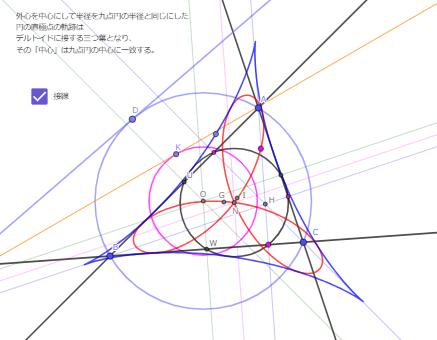
①This example demonstrates the locus of the orthopole of a moving point P on a circle centered at the circumcenter O of a triangle ABC. The orthopole is defined as the point where the perpendiculars from P to the three sides of the triangle are concurrent (or their feet are collinear). ②Core mathematical concepts include the circumcenter, orthopole, pedal points, collinearity, and locus generation, integrating circles, lines, perpendiculars, and parallels. ③Construction uses GeoGebra commands: TriangleCenter to get O, Line and Circle for the base circle, Point for the moving P, Tangent, OrthogonalLine, Intersect to build perpendiculars and intersections, and Locus to trace the orthopole path, with auxiliary tools like LineBisector and Distance. ④Suitable for high school or university geometry courses, exploring pole-polar theory related to triangles and circles, and dynamic locus visualization.
GeoGebra Commands & Parameters
TriangleCenter(A, B, C, 3) → OLine(A, B) → fLine(B, C) → gLine(C, A) → hCircle(B, C, A) → cPoint(c) → DTangent(D, c) → i,OrthogonalLine(A, i) → jOrthogonalLine(C, i) → kOrthogonalLine(B, i) → lIntersect(i, l) → EIntersect(i, j) → FIntersect(i, k) → G_1OrthogonalLine(E, h) → mOrthogonalLine(F, g) → pOrthogonalLine(G_1, f) → nIntersect(m, p) → H_1TriangleCenter(A, B, C, 4) → HTriangleCenter(A, B, C, 1) → ITriangleCenter(A, B, C, 5) → NOrthogonalLine(P, g) → q_1Intersect(g, q_1) → WCircle(P, Distance[W, N]) → dPoint(d) → KTangent(K, d) → q, n_1OrthogonalLine(A, q) → rOrthogonalLine(C, q) → sOrthogonalLine(B, q) → tIntersect(r, q) → LIntersect(q, s) → MIntersect(t, q) → N_1OrthogonalLine(L, g) → bOrthogonalLine(M, f) → eOrthogonalLine(N_1, h) → f_1Intersect(e, f_1) → O_1TriangleCenter(A, B, C, 2) → GLocus(O_1, K) → loc1Locus(H_1, D) → loc2Point(c) → JLine(P, J) → g_1OrthogonalLine(A, g_1) → h_1OrthogonalLine(B, g_1) → i_1Intersect(g_1, h_1) → RIntersect(g_1, i_1) → SOrthogonalLine(S, h) → k_1OrthogonalLine(R, g) → m_1OrthogonalLine(C, g_1) → j_1Intersect(g_1, j_1) → QOrthogonalLine(Q, f) → l_1Intersect(k_1, m_1) → TOrthogonalLine(P, f) → p_1OrthogonalLine(P, h) → r_1Intersect(f, p_1) → UIntersect(r_1, h) → VCircle(U, W, V) → c_1LineBisector(U, W) → s_1LineBisector(U, V) → t_1Distance(W, N) → distanceWNIntersect(c_1, g, 2) → A_1Intersect(c_1, h, 2) → B_1Intersect(c_1, f, 2) → C_1OrthogonalLine(C_1, f) → a_1OrthogonalLine(A_1, g) → b_1OrthogonalLine(B_1, h) → d_1Intersect(a_1, d_1) → D_1
AI Drawing Prompt Reference
Construct a triangle ABC and use its circumcenter O as reference. Draw the three side lines AB, BC, and CA, and the circle passing through B, C, and A. Let a moving point P travel on this circle. From P, draw perpendiculars to the three sides to realize the orthopole definition (the three perpendicular feet/concurrency condition). Using intersections from these perpendicular lines, construct the orthopole point K corresponding to each position of P. Then trace the locus of K as P moves along the circle; optionally show a second auxiliary locus coming from the same orthopole-type construction to emphasize the geometric relationship.
The prompt above was compiled from the original drawing commands and is for reference only.