
Lissajous Curve as a Sinusoid Rolled on a Cylinder
Loading the math board and drawing, please wait…
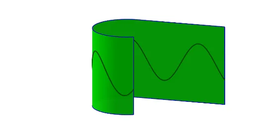
① This example demonstrates the geometric equivalence between a Lissajous curve and a sinusoid rolled on a cylinder, visualizing how a 2D parametric curve emerges from a 3D construction. ② Core mathematical concepts include parametric equations, sine functions, cylindrical surfaces, curve-surface interaction, and the influence of frequency ratio and phase difference on the Lissajous shape. ③ Construction highlights: using GeoGebra commands such as Sequence, CurveCartesian, Surface, Segment, and Midpoint, with parameters like amplitude (Amp), radius (r), expansion (Expand), height (h), frequency ratio (n), and phase (phase), all adjustable via sliders to animate the curve. ④ Suitable for high school to undergraduate mathematics education, particularly for exploring analytic geometry, trigonometry, and parametric equations, as well as demonstrating the relationship between 3D curves and their 2D projections.
GeoGebra Commands & Parameters
Sequence(((-If[Expand ≤ 0.5, (((Expand * 2) * π) * r), (π * r)]) + If[t ≤ ((Expand * 2) * π), (t * r), (((Expand * 2) * π) * r) + (r * sin(t - ((Expand * 2) * π)))], (-r) + If[t ≤ ((Expand * 2) * π), 0, r - (r * cos(t - ((Expand * 2) * π)))], h / 2), t, 0, (2 * π), (2 * π / n)) → l1CurveCartesian((-If[Expand ≤ 0.5, (((Expand * 2) * π) * r), (π * r)]) + If[t ≤ ((Expand * 2) * π), (t * r), (((Expand * 2) * π) * r) + (r * sin(t - ((Expand * 2) * π)))], (-r) + If[t ≤ ((Expand * 2) * π), 0, r - (r * cos(t - ((Expand * 2) * π)))], t, 0, (2 * π)) → aCurveCartesian((-If[Expand ≤ 0.5, (((Expand * 2) * π) * r), (π * r)]) + If[t ≤ ((Expand * 2) * π), (t * r), (((Expand * 2) * π) * r) + (r * sin(t - ((Expand * 2) * π)))], (-r) + If[t ≤ ((Expand * 2) * π), 0, r - (r * cos(t - ((Expand * 2) * π)))], h, t, 0, (2 * π)) → cSurface((-If[Expand ≤ 0.5, (((Expand * 2) * π) * r), (π * r)]) + If[t ≤ ((Expand * 2) * π), (t * r), (((Expand * 2) * π) * r) + (r * sin(t - ((Expand * 2) * π)))], (-r) + If[t ≤ ((Expand * 2) * π), 0, r - (r * cos(t - ((Expand * 2) * π)))], s, t, 0, (2 * π), s, 0, h) → bSegment(((-If[Expand ≤ 0.5, (((Expand * 2) * π) * r), (π * r)]), (-r) + 0, 0), ((-If[Expand ≤ 0.5, (((Expand * 2) * π) * r), (π * r)]), (-r) + 0, h)) → fSegment(((-If[Expand ≤ 0.5, (((Expand * 2) * π) * r), (π * r)]) + (((Expand * 2) * π) * r) + (r * sin((2 * π) - ((Expand * 2) * π))), (-r) + r - (r * cos((2 * π) - ((Expand * 2) * π))), 0), ((-If[Expand ≤ 0.5, (((Expand * 2) * π) * r), (π * r)]) + (((Expand * 2) * π) * r) + (r * sin((2 * π) - ((Expand * 2) * π))), (-r) + r - (r * cos((2 * π) - ((Expand * 2) * π))), h)) → gSegment((0, (-r), 0), (0, (-r), h)) → iSequence(Element[l1, i] + (0, 0, (Amp * sin(((0.1 * w) * i) - 1 + phase))), i, 1, Length[l1]) → l2Midpoint(f) → AMidpoint(g) → BMidpoint(A, B) → CSequence(Segment[Element[l2, i], Element[l2, i + 1]], i, 1, Length[l2]) → l3
AI Drawing Prompt Reference
Draw a Lissajous curve demonstrating its geometric equivalence to a sinusoid rolled on a cylinder. The curve is defined by parametric equations with adjustable amplitude, radius, height, frequency ratio, and phase difference. First, visualize the 3D representation of the curve, then plot its 2D projection onto the xy-plane. Connect the start and end points of the projection with line segments, and draw a line segment between their midpoints. Finally, link consecutive points on the projection with line segments to form a continuous curve.
The prompt above was compiled from the original drawing commands and is for reference only.