
Linear vs. Angular Speed: Geometric and Motion Analysis
Loading the math board and drawing, please wait…
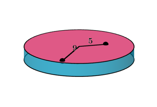
This example demonstrates the comparison between linear and angular speed using geometric diagrams. Key mathematical concepts include speed formulas, geometric interpretations of rotation and translation, and how to represent speed changes using coordinate systems and graphs. Construction involves using GeoGebra objects such as circles, lines, points, and segments. Suitable for high school or university students learning kinematics and geometric applications.
GeoGebra Commands & Parameters
Circle((0, 0, 0), (2, 0, 0), zAxis) → cTranslate(c, Vector[(0, 0, 0.5)]) → c'Surface((2 * cos(u)), (2 * sin(u)), v, u, 0, (2 * π), v, 0, 0.5) → aCircle((0, 0, 1 / 2), 1.8, zAxis) → eCircle((0, 0, 1 / 2), 1, zAxis) → dPoint(d) → APoint(e) → BSegment(C, A) → fSegment(C, B) → g
AI Drawing Prompt Reference
Create a 3D geometric model illustrating linear vs. angular speed. Start with a circle of radius 2 centered at the origin in the horizontal plane, then translate it vertically by 0.5 units to form a cylindrical side surface. Inside the cylinder, at height 0.5, place two concentric circles with radii 1.8 and 1. Pick one point on each of these circles, and draw two line segments from the center point of the cylinder's base to each of these points. The final figure shows a cylinder, concentric circles, and connecting segments for analyzing rotational and translational speed relationships.
The prompt above was compiled from the original drawing commands and is for reference only.