Linear Regression Slopes: Dynamic Demonstration with Random Data

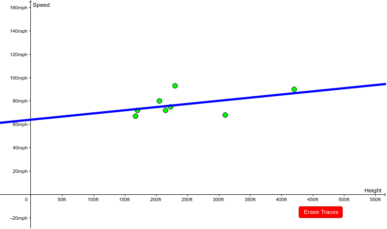
This GeoGebra example dynamically demonstrates the concept of slope in linear regression. It generates a set of random data points, fits a least-squares regression line, and displays the slope of that line. Core mathematical concepts include linear regression, least squares method, slope, and data fitting. Construction highlights: uses Shuffle and Sequence commands to generate random data points, FitLineY to compute the regression line, and Slope to extract its slope; objects include data points A1-B8, variables height and speed, lists list1 and data, fitted function f, parameters a and n, and a button (button1) for interactive control. Suitable for high school or college courses in statistics and data analysis to illustrate regression principles, and for math lab sessions to help students intuitively grasp how the slope affects the fit.