
Linear Regression by Jed Butler
Loading the math board and drawing, please wait…
In collections
GGBChat4: Statistics 1
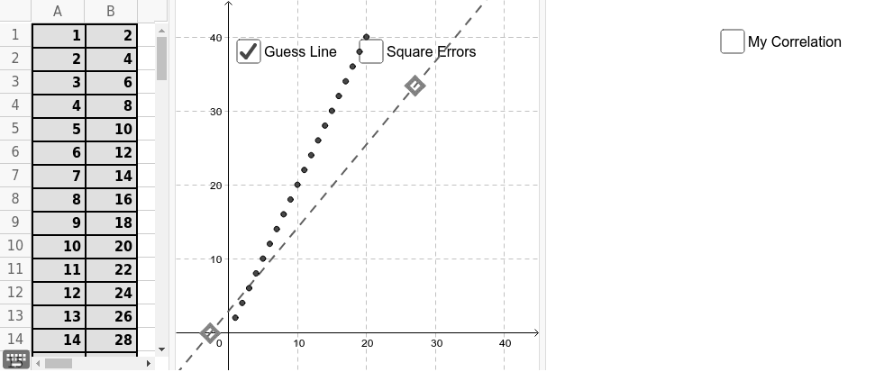
This example demonstrates how users can define points by dragging or manually inputting/modifying them in a spreadsheet, and then plot a scatter plot along with the fitted linear regression line. Key math concepts include linear regression, correlation coefficient, least squares method, and analytical geometry. The construction involves commands/objects like Line, Intersect, Polygon, Vector, RSquare, SampleSD, Median, Text, FitLineY, and Circle as per the GeoGebra command summary. Suitable for high school and above learners to understand data fitting and statistical analysis methods.
GeoGebra Commands & Parameters
Line(U, V) → line_{guess}Line(A, x = 0) → aLine(B, x = 0) → bLine(C, x = 0) → cLine(D, x = 0) → dLine(E, x = 0) → eLine(F, x = 0) → fLine(G, x = 0) → gLine(H, x = 0) → hLine(I, x = 0) → iLine(J, x = 0) → jLine(K, x = 0) → kLine(L, x = 0) → lLine(M, x = 0) → mLine(N, x = 0) → nLine(NP, x = 0) → npLine(O, x = 0) → pLine(P, x = 0) → qLine(R, x = 0) → sLine(S, x = 0) → tIntersect(line_{guess}, a) → A'Intersect(line_{guess}, b) → B'Intersect(line_{guess}, c) → C'Intersect(line_{guess}, d) → D'Intersect(line_{guess}, e) → E'Intersect(line_{guess}, f) → F'Intersect(line_{guess}, g) → G'Intersect(line_{guess}, h) → H'Intersect(line_{guess}, i) → I'Intersect(line_{guess}, j) → J'Intersect(line_{guess}, k) → K'Intersect(line_{guess}, l) → L'Intersect(line_{guess}, m) → M'Intersect(line_{guess}, n) → N'Intersect(line_{guess}, np) → NP'Intersect(line_{guess}, p) → O'Intersect(line_{guess}, q) → P'Intersect(line_{guess}, s) → R'Intersect(line_{guess}, t) → S'Line(Q, x = 0) → rIntersect(line_{guess}, r) → Q'Polygon(A', A, 4) → poly1, a_1, b_1, c_1, d_1, T, WPolygon(B', B, 4) → poly2, e_1, f_1, g_1, h_1, Z, A_1Polygon(D', D, 4) → poly3, i_1, j_1, k_1, l_1, B_1, C_1Polygon(E', E, 4) → poly4, m_1, n_1, p_1, q_1, D_1, E_1Polygon(C', C, 4) → poly5, r_1, s_1, t_1, a_2, F_1, G_1Polygon(F', F, 4) → poly6, b_2, c_2, d_2, e_2, H_1, I_1Polygon(G', G, 4) → poly7, f_2, g_2, h_2, i_2, J_1, K_1Polygon(H', H, 4) → poly8, j_2, k_2, l_2, m_2, L_1, M_1Polygon(I', I, 4) → poly9, n_2, p_2, q_2, r_2, N_1, O_1Polygon(J', J, 4) → poly10, s_2, t_2, a_3, b_3, P_1, Q_1Polygon(K', K, 4) → poly11, c_3, d_3, e_3, f_3, R_1, S_1Polygon(L', L, 4) → poly12, g_3, h_3, i_3, j_3, T_1, U_1Polygon(M', M, 4) → poly13, k_3, l_3, m_3, n_3, V_1, W_1Polygon(N', N, 4) → poly14, p_3, q_3, r_3, s_3, Z_1, A_2Polygon(NP', NP, 4) → poly15, t_3, a_4, b_4, c_4, B_2, C_2Polygon(P', P, 4) → poly16, d_4, e_4, f_4, g_4, D_2, E_2Polygon(O', O, 4) → poly17, h_4, i_4, j_4, k_4, F_2, G_2Polygon(Q', Q, 4) → poly18, l_4, m_4, n_4, p_4, H_2, I_2Polygon(R', R, 4) → poly19, q_4, r_4, s_4, t_4, J_2, K_2Polygon(S', S, 4) → poly20, a_5, b_5, c_5, d_5, L_2, M_2Vector((x(A), 0), (x(A), y(A) - y(A'))) → V_AVector((x(B), 0), (x(B), y(B) - y(B'))) → V_BVector((x(C), 0), (x(C), y(C) - y(C'))) → V_CVector((x(D), 0), (x(D), y(D) - y(D'))) → V_DVector((x(E), 0), (x(E), y(E) - y(E'))) → V_EVector((x(F), 0), (x(F), y(F) - y(F'))) → V_FVector((x(G), 0), (x(G), y(G) - y(G'))) → V_GVector((x(H), 0), (x(H), y(H) - y(H'))) → V_HVector((x(I), 0), (x(I), y(I) - y(I'))) → V_IVector((x(J), 0), (x(J), y(J) - y(J'))) → V_JVector((x(K), 0), (x(K), y(K) - y(K'))) → V_KVector((x(L), 0), (x(L), y(L) - y(L'))) → V_LVector((x(M), 0), (x(M), y(M) - y(M'))) → V_MVector((x(N), 0), (x(N), y(N) - y(N'))) → V_NVector((x(NP), 0), (x(NP), y(NP) - y(NP'))) → V_{NP}Vector((x(P), 0), (x(P), y(P) - y(P'))) → V_PVector((x(Q), 0), (x(Q), y(Q) - y(Q'))) → V_QVector((x(R), 0), (x(R), y(R) - y(R'))) → V_RVector((x(O), 0), (x(O), y(O) - y(O'))) → V_OVector((x(S), 0), (x(S), y(S) - y(S'))) → V_SRSquare(data, line_{guess}) → StrengthSampleSD(list_y) → SD_yMedian(list_x) → Median_xVector((Median_x / 2, (SD_y * 2)), (Median_x / 2, (SD_y * 2) + over)) → Vector_{over}Vector((Median_x / 2, (SD_y * 2)), (Median_x / 2, (SD_y * 2) - under)) → Vector_{under}Text(((Strength * 100) * "%"), ((Median_x * 1.425), (SD_y * 1.95))) → text1FitLineY(data) → line_{actual}Circle(((Median_x * 1.5), (2 * SD_y)), (Strength * Max[list_y] / 6)) → g_5Circle(((Median_x * 1.5), (2 * SD_y)), (Strength * Max[list_y] / 6)) → CorrelationCircleCircle(((Median_x * 1.5), (2 * SD_y)), (Strength * Max[list_y] / 6)) → CorrelationCircle_1Circle(((Median_x * 1.5), (2 * SD_y)), (Strength * Max[list_y] / 6)) → f_5
AI Drawing Prompt Reference
Draw a scatter plot with multiple points and fit a linear regression line. First, define points by dragging or manual input, then plot them in the coordinate system. Next, calculate and draw the best-fit line passing through these points to demonstrate linear regression. Finally, enclose the points with several quadrilaterals to highlight the data distribution characteristics.
The prompt above was compiled from the original drawing commands and is for reference only.