Linear Programming & Geometric Transformations Demo

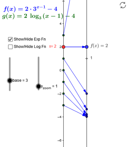
This example dynamically demonstrates linear programming, showing how the optimal solution of an objective function within a feasible region is determined through geometric transformations (translation, rotation). Key math concepts include linear programming, feasible region, objective function, vector, and geometric transformations. GeoGebra commands and objects like Point, Vector, Textfield, and Sequence are used to create and interact with geometric elements. Suitable for high school and above learners to understand the intuitive representation of abstract optimization problems.