Linear Equation Slope Y-Intercept Demo

Loading the math board and drawing, please wait…

2017-11-22 00:37

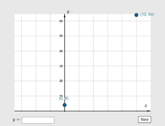
This example demonstrates the graph of a linear equation y=mx+b and the relationship between its slope m and y-intercept b. Core math concepts include linear functions, slope, y-intercept, and coordinate geometry. Construction highlights involve GeoGebra commands/objects like Random, RandomElement, Max, Min, If, Polygon, Textfield, Vector, and elements such as clist, b, d, a, A, c, B, xmin, xmax, p, ymax, ymin, f, yscale, C1, C2, C3, C4, q1, InputBox1, button1, g, answer, text1, text2, text3, v, text4, u. Suitable for high school mathematics education to understand the impact of parameter changes on the graph.

GeoGebra Commands & Parameters

Random(-2, 20) → b
Random(-5, 7) → d
RandomElement(clist) → c
Max({y(A) + 10, y(B) + 10, 10}) → ymax
Min({y(A) - 10, y(B) - 10, -10}) → ymin
If((ymax - ymin) / 9 < 10, (ymax - ymin) / 9, If[(ymax - ymin) / 10 < 10, (ymax - ymin) / 10, (ymax - ymin) / 12]) → yscale
Polygon({C1, C2, C3, C4}) → q1
Textfield(f) → InputBox1
Vector((0, ymax - (1.5 * yscale)), (0, ymax - yscale)) → v
Vector((10, 0), (12, 0)) → u

AI Drawing Prompt Reference

Create a demonstration graph of a linear equation y=mx+b, showing the relationship between slope and y-intercept. The graph includes a straight line whose slope and intercept are randomly generated, with an input box for the function expression. The coordinate axes are scaled automatically based on two key points on the line, with appropriate tick spacing. Add a text field above the graph for entering or displaying the equation. Also draw two arrow vectors: one vertical pointing upward near the y-axis, and one horizontal pointing right along the x-axis, to indicate axis directions. The layout is clear and suitable for high school students to explore how changing parameters affects the line.

The prompt above was compiled from the original drawing commands and is for reference only.