
Line Integrals of Vector Fields: Work & Circulation
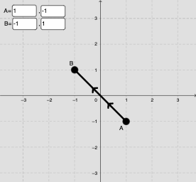
Loading the math board and drawing, please wait…
This example illustrates the concept of line integrals in vector fields, including work and circulation. By constructing vector fields, path integrals, and geometric shapes, students can gain a visual understanding of these concepts. GeoGebra commands such as SelectedIndex, Midpoint, and Derivative are used. Suitable for university mathematics and physics courses.
GeoGebra Commands & Parameters
SelectedIndex(pathNames) → pathIndexMidpoint(N, P) → QElement(pathList, pathIndex) → pathDerivative(path) → DDpathParametricDerivative(path) → DpathDistance(N, P) → NPElement(CompX, pathIndex) → RTXDerivative(RTX, x) → DRTXElement(CompY, pathIndex) → RTYDerivative(RTY, x) → DRTYCurveCartesian(x(path(t)), y(path(t)), t, 0, s) → partPathIntegral(MUL, 0, 1) → WorkTextfield(F_1) → InputBox1Textfield(F_2) → InputBox2Segment(path(0.3), path(0.3 + 0.01)) → arrow1Segment(path(0.6), path(0.6 + 0.01)) → arrow2If(Work ≟ Work, Work, Sum[Sequence[((path(i + dS) - path(i)) * (F_1(x(path(i + dS / 2)), y(path(i + dS / 2))), F_2(x(path(i + dS / 2)), y(path(i + dS / 2))))), i, 0, s - dS, dS]]) → WOORKSequence(Vector[path(i), path(i) + ((scale * F_1(x(path(i)), y(path(i)))), (scale * F_2(x(path(i)), y(path(i)))))], i, 0, s, 0.15) → PathVectorsSequence(path(i), i, 0.25, 0.75, 0.25) → PtPathListSequence(Vector[(0, 0), (1 / sqrt((y(DDpath(i)))^(2) + (x(DDpath(i)))^(2)) * (x(DDpath(i)), y(DDpath(i))))], i, 0.25, 0.75, 0.25) → tangvectorsListTranslate(Vector[Element[tangvectorsList, 1]], Element[PtPathList, 1]) → uuTranslate(Vector[Element[tangvectorsList, 2]], Element[PtPathList, 2]) → vvTranslate(Vector[Element[tangvectorsList, 3]], Element[PtPathList, 3]) → wwTextfield(xA) → InputBox3Textfield(yA) → InputBox4Textfield(xB) → InputBox5Textfield(yB) → InputBox6
AI Drawing Prompt Reference
Visualize line integrals in vector fields, showing work and circulation. Construct vector fields, path integrals, and geometric shapes. Mark midpoints and tangent vectors on the path, and represent vector field directions with arrows. Finally, calculate and display the results of the line integral, distinguishing work and circulation with different colors.
The prompt above was compiled from the original drawing commands and is for reference only.