Line Integral of a Vector Field in 3-Space

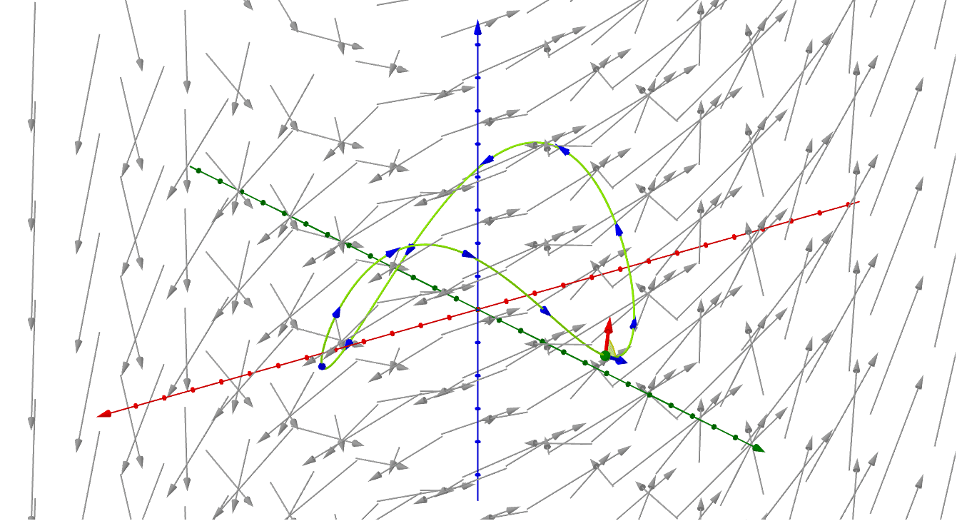
This GeoGebra example visualizes the line integral of a vector field along a space curve in three dimensions. It dynamically shows the dot product between the vector field and the tangent vector at each point on the path, making the geometric meaning of the line integral clear. Core mathematical concepts include vector fields, parametric curves, tangent vectors, dot products, and the definition and computation of line integrals. The construction uses the CurveCartesian command to define a 3D parametric curve, Derivative to obtain the tangent vector, Sequence and Vector to sample the vector field and tangent vectors along the path, and Angle to display the angle between them. A slider t_0 controls the upper limit of integration, updating the cumulative integral value C_v in real time. This example is suitable for university-level calculus or multivariable calculus courses, and can also be used to intuitively teach concepts like work and circulation in mathematical physics.