
Line Gradient Self Quiz
Loading the math board and drawing, please wait…
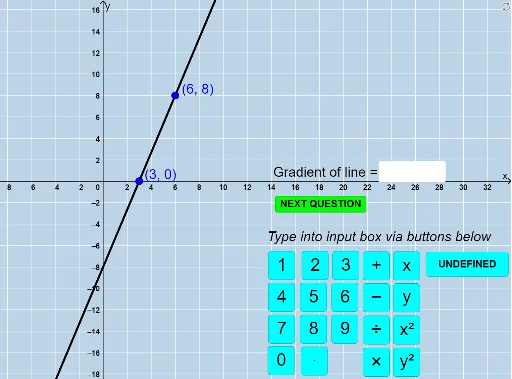
This example demonstrates how to dynamically illustrate the calculation and properties of line gradients using GeoGebra. The core mathematical concepts involved include the definition of slope, linear equations, vector operations, and geometric transformations. Key construction points—extracted from the «Construction Summary» below—utilize GeoGebra commands/objects such as GCD (Greatest Common Divisor), If (Conditional Judgment), OrthogonalLine (Perpendicular Line), Intersect (Intersection), Line (Line), Polygon (Polygon), Distance (Distance), Segment (Segment), Angle (Angle), Slope (Slope), Dilate (Dilation), Vector (Vector), Random (Random Number), Textfield (Text Field), RandomElement (Random Element), etc. It is suitable for middle school students and above to learn and review concepts related to slope in analytical geometry.
GeoGebra Commands & Parameters
GCD(deltaY, deltaX) → GCDmGCD(numerYint, deltaX) → GCDyIf(sgn(deltaY / deltaX) ≥ 0, "", "-") → textSignNIf(sgn(numerYint / deltaX) > 0, "+", "-") → textSignIf(deltaXR ≟ 1, textSignN + deltaYR, textSignN + "\, \frac{" + deltaYR + "}{" + deltaXR + "}") → textslopeNIf(denomYintR ≟ 1, textSign + numerYintR, textSign + "\frac{" + numerYintR + "}{" + denomYintR + "}") → textYintIf(denomYintR ≟ 1, If[numerYintR ≟ 1, textSign, textSign + numerYintR], textSign + "\frac{" + numerYintR + "}{" + denomYintR + "}") → textMIDOrthogonalLine(B, xAxis) → a_2OrthogonalLine(A, yAxis) → cIntersect(a_2, c) → CLine(A, B) → dPolygon(A, B, C) → poly1, c_1, a_1, b_1Distance(B, C) → distanceBCDistance(A, C) → distanceACIntersect(a_2, c) → DSegment(A, D) → eSegment(C, B) → fGCD(deltaY_1, deltaX_1) → GCDm_1If(sgn(deltaY_1 / deltaX_1) ≥ 0, "", "-") → textSignN_1If(deltaXR_1 ≟ 1, textSignN_1 + deltaYR_1, textSignN_1 + "\, \frac{" + deltaYR_1 + "}{" + deltaXR_1 + "}") → textslopeN_1Line(A_1, B_1) → d_1Angle(B, D, A) → αSegment(A, B) → gGCD(deltaY_2, deltaX_2) → GCDm_2If(sgn(deltaY_2 / deltaX_2) ≥ 0, "", "-") → textSignN_2If(deltaXR_2 ≟ 1, textSignN_2 + deltaYR_2, textSignN_2 + "\, \frac{" + deltaYR_2 + "}{" + deltaXR_2 + "}") → textslopeN_2Line(A_2, B_2) → d_2Segment(A_2, B_2) → g_1GCD(deltaY_3, deltaX_3) → GCDm_3If(sgn(deltaY_3 / deltaX_3) ≥ 0, "", "-") → textSignN_3If(deltaXR_3 ≟ 1, textSignN_3 + deltaYR_3, textSignN_3 + "\, \frac{" + deltaYR_3 + "}{" + deltaXR_3 + "}") → textslopeN_3Line(A_3, B_3) → d_3Segment(A_3, B_3) → g_2Slope(g) → hDilate(A, If[0 < i ≤ 1, 1 - i, 0], D) → A'Vector(A, A') → uDilate(D, If[1 < i ≤ 2, 2 - i, 0], B) → D'Vector(D, D') → vLine(A, B) → jRandom(-6, 6) → randomXBRandom(-8, 8) → randomXARandom(-5, 5) → randomYATextfield(textanswer) → InputBox1If(abs(answergradient - gradientLine) < 0.005, true, If[x(A) ≟ x(B), If[textanswer ≟ "undefined" ∨ textanswer ≟ "Undefined" ∨ textanswer ≟ "UNDEFINED", true, false]]) → answercorrectRandomElement({0, 2, 3, 4, 5, 6, 7, 8}) → randomdeltay_BIf(randomXA ≟ randomXB ∧ randomdeltay_B ≟ 0, 5, 0) → addXB
AI Drawing Prompt Reference
Draw a dynamic illustration showing the calculation and properties of line gradients, including two lines and their intersection points, displaying the slope formula and y-intercept, highlighting key points and vectors with different colors, and add a random line with an input box for users to calculate the slope, which will be highlighted when correct.
The prompt above was compiled from the original drawing commands and is for reference only.