
Limits for Complex Functions
Loading the math board and drawing, please wait…
In collections
Mapping Diagrams to Visualize Complex Analysis
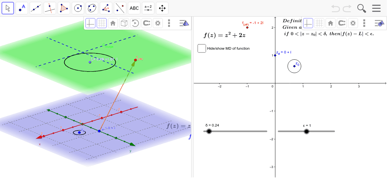
This example demonstrates the geometric visualization of limits for complex functions. Using GeoGebra commands like Sequence, CurveCartesian, and PointIn, it constructs points, line segments, and circles to illustrate the limit process. The key mathematical concepts involve complex numbers, limits, and geometric construction. The construction steps include using vectors, points, circles, and curves to build the limit graph. This is suitable for high school students or college undergraduates learning the basics of complex numbers and calculus.
GeoGebra Commands & Parameters
Sequence((δ * (cos(t) + (sin(t) * ί))) + x(z_0) + (y(z_0) * ί), t, -3.14159, 3.141592653589793, 0.5236) → z_*Sequence((x(Element[fz_*, k]), y(Element[fz_*, k]), height_{image}), k, 1, 12) → fpoint_*Sequence(Vector[Element[z_*, j], Element[fpoint_*, j]], j, 1, 12) → fvec_*CurveCartesian((δ * cos(t)), (δ * sin(t)), height_{image}, t, 0, 6.283185307179586) → dTextfield(fz_*) → inputBox1Vector(z_#, f_{(z#).}) → wTextfield(f_{(z#)}) → inputBox2CurveCartesian(t, 0, height_{image}, t, -5, 5) → XhCurveCartesian(0, t, height_{image}, t, -5, 5) → YhTextfield(z_*) → inputBox3PointIn(C_{image}) → LCircle(L, ε, Vector[(0, 0, 1)]) → f
AI Drawing Prompt Reference
Draw a graph of the limit of a complex function. Start by generating a series of points using the complex number δ(cos(t) + sin(t)i) around a central point z_0. Then, use these points to draw a series of vectors fvec_* and construct a curve d with points fpoint_*. Next, input function values fz_* via inputBox1 and draw a resizable circle f in the image. Finally, input vectors via inputBox2 to show vectors from points z_* to f. Also, draw X and Y axes as references.
The prompt above was compiled from the original drawing commands and is for reference only.