
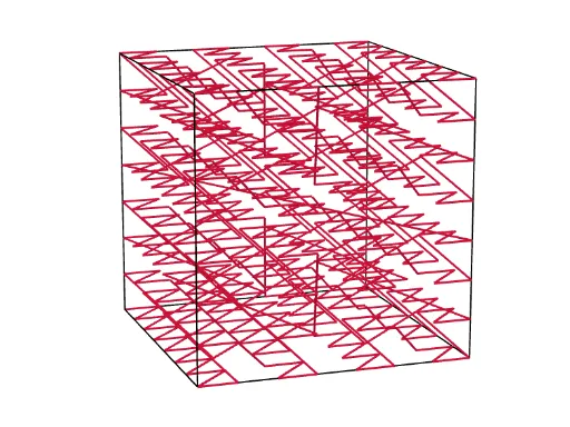
Lebesgue 3D Curves Visualization
Loading the math board and drawing, please wait…
This example demonstrates the construction and visualization of Lebesgue 3D curves. It involves core mathematical concepts like solid geometry, parametric equations, and vector analysis. The construction uses GeoGebra commands such as Point, Cube, PolyLine, Sequence, and Flatten. Suitable for high school students and math enthusiasts studying 3D curves and spatial geometry.
GeoGebra Commands & Parameters
Point(Circle[B, Distance[A, B], Segment[A, B]]) → CCube(A, B, C) → a, D, faceCDHG, faceEFGH, edgeAD, edgeAB_1, edgeBC, edgeCD, edgeAE, edgeDH, edgeEH, edgeEF, E, edgeBF, edgeFG, edgeCG, edgeGH, F, G, H, faceABCD, faceADHE, faceABFE, faceBCGFPolyLine(l1) → fSequence(Dilate[l1, 1 / 3, l1(w)], w, 1, 8) → l2PolyLine(Flatten[l2]) → gFlatten(l2) → l3Sequence(Dilate[l3, 3 / 7, l1(w)], w, 1, 8) → l4PolyLine(Flatten[l4]) → hFlatten(l4) → l5Sequence(Dilate[l5, 7 / 15, l1(w)], w, 1, 8) → l6PolyLine(Flatten[l6]) → iPoint(Circle[B, Distance[A, B], Segment[A, B]]) → ICube(A, B, I) → c, J, faceIJNM, faceKLMN, edgeAJ, edgeAB, edgeBI, edgeIJ, edgeAK, edgeJN, edgeKN, edgeKL, K, edgeBL, edgeLM, edgeIM, edgeMN, L, M, N, faceABIJ, faceAJNK, faceABLK, faceBIML