
Lagrange Multipliers Example 8: Constrained Optimization on a 3D Surface
Loading the math board and drawing, please wait…
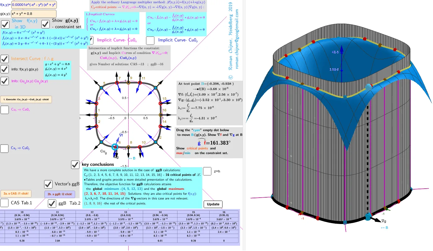
① This example visually demonstrates the method of Lagrange multipliers for finding extrema of a function subject to a constraint, showing the intersection of the objective surface with a constraint cylinder and the optimal point. ② Core mathematical concepts include multivariable optimization, Lagrange multipliers, gradient vectors, constraint curves, tangent planes, and solving systems of partial derivative equations. ③ Construction highlights: Based on the construction summary, GeoGebra commands such as CurveCartesian (parametric curves), Surface, Point, Vector, Segment, and Text are used, with functions f (objective) and g (constraint) and their partial derivatives fx', fy', gx', gy' defined; gradient vectors Vf and Vg, Lagrange multipliers l1 and l2, interactive buttons (button4, etc.), and a slider (α) are included for dynamic exploration. ④ Suitable for university-level calculus or advanced mathematics courses explaining conditional extrema, and useful for teaching mathematical modeling or engineering optimization, helping students grasp both the geometric intuition and algebraic solution of Lagrange multipliers.
GeoGebra Commands & Parameters
Simplify(Derivative[f, y, 1]) → fy'Simplify(Derivative[f, x, 1]) → fx'LeftSide(Cu_g) → gSimplify(Derivative[g, y, 1]) → gy'Simplify(Derivative[g, x, 1]) → gx'Point(Cu_g) → BVector(B, B + UnitVector[Vector[B, Dg]] / 3) → u_gVector(B, B + UnitVector[Vector[B, Df]] / 3) → u_fAngle(u_g, u_f) → αLaTeX(f, true) → text8aLaTeX(Cu_g, true) → text8bTextfield(f) → InputBox3Textfield(Cu_g) → InputBox4CurveCartesian(sqrt(cos(t)), (0.8 - cos(t)^(2))^(0.25), f(sqrt(cos(t)), (0.8 - cos(t)^(2))^(0.25)), t, (-π), π) → q1CurveCartesian((-sqrt(cos(t))), (0.8 - cos(t)^(2))^(0.25), f(sqrt(cos(t)), (0.8 - cos(t)^(2))^(0.25)), t, (-π), π) → q2CurveCartesian(sqrt(cos(t)), (-(0.8 - cos(t)^(2))^(0.25)), f(sqrt(cos(t)), (-(0.8 - cos(t)^(2))^(0.25))), t, (-π), π) → q1aCurveCartesian((-sqrt(cos(t))), (-(0.8 - cos(t)^(2))^(0.25)), f((-sqrt(cos(t))), (-(0.8 - cos(t)^(2))^(0.25))), t, (-π), π) → q2aTextfield(n) → InputBox5Element(l1, Indexmax1) → Amax1Element(l2, Indexmax2) → Amax2Element(l1, Indexmin1) → Amin1Element(l2, Indexmin2) → Amin2Element(l1f, Indexmax1) → Amax1_{3D}Element(l2f, Indexmax2) → Amax2_{3D}Element(l1f, Indexmin1) → Amin1_{3D}Element(l2f, Indexmin2) → Amin2_{3D}LaTeX(Amin2_{3D}, true, true) → text17Zip(ScientificText[a, 4], a, z(l2f)) → l2faZip(ScientificText[a, 4], a, z(l1f)) → l1faTableText(Append["N", 1…Length[l2]], Append["\fgcolor{red}{Cp}", l2], Append["\fgcolor{blue}{f}(\fgcolor{red}{C_p })", l2fa], Append["(\dot{f_x},\dot{f_y})", l2xy'_fa], Append["(\dot{g_x},\dot{g_y})", l2xy'_ga], Append["λ_x", lλ2ax], Append["λ_y", lλ2ay], Append["\widehat{\dot{g}\dot{f}} ", lα2], "c|_") → tTab2TableText(Append["N", 1…Length[l1]], Append["\fgcolor{red}{Cp}", l1], Append["\fgcolor{blue}{f}(\fgcolor{red}{C_p })", l1fa], Append["(\dot{f_x},\dot{f_y})", l1xy'_fa], Append["(\dot{g_x},\dot{g_y})", l1xy'_ga], Append["λ_x", lλ1ax], Append["λ_y", lλ1ay], Append["\widehat{\dot{g}\dot{f}} ", lα1], "c|_") → tTab1Segment(B, C) → f_1Text("∇f", Point[u_f, 1]) → text25fRotateText(text14, 90°) → text15Text("∇g", Point[u_g, 1]) → text25gSequence(If[lα1(i) ≟ 180°, 1, lα1(i) ≟ 0° ∨ lα1(i) ≟ 360°, 2, 3], i, 1, Length[l1]) → l1_αSurface(((-0.8^(0.25)) * (1 - sin(t)^(4))^(0.25)), (0.8^(0.25) * sin(t)), u, t, 0, (2 * π), u, 0, (4 * 10^(-6))) → g02Surface((0.8^(0.25) * (1 - sin(t)^(4))^(0.25)), (0.8^(0.25) * sin(t)), u, t, (-π), π, u, 0, (4 * 10^(-6))) → g01Surface(sqrt(cos(t)), (0.8 - cos(t)^(2))^(0.25), u, t, (-π), π, u, 0, (4 * 10^(-6))) → g1Surface((-sqrt(cos(t))), (0.8 - cos(t)^(2))^(0.25), u, t, (-π), π, u, 0, (4 * 10^(-6))) → g2Surface(sqrt(cos(t)), (-(0.8 - cos(t)^(2))^(0.25)), u, t, (-π), π, u, 0, (4 * 10^(-6))) → g1aSurface((-sqrt(cos(t))), (-(0.8 - cos(t)^(2))^(0.25)), u, t, (-π), π, u, 0, (4 * 10^(-6))) → g2aRemoveUndefined(Zip[If[(abs(x(A)) * 10^(15)) < 1 ∧ (abs(y(A)) * 10^(15)) < 1, b, (NaN, NaN)], A, l1xy'_f, b, l1]) → l1_{loc}RemoveUndefined(Zip[If[(abs(x(l2xy'_f(k))) * 10^(14)) < 1 ∧ (abs(y(l2xy'_f(k))) * 10^(14)) < 1, k, NaN], k, 1…Length[l2]]) → l2_{loc}NRemoveUndefined(Zip[If[(abs(x(l1xy'_f(k))) * 10^(14)) < 1 ∧ (abs(y(l1xy'_f(k))) * 10^(14)) < 1, k, NaN], k, 1…Length[l1]]) → l1_{loc}NRemoveUndefined(Sequence[If[lα1(i) ≟ 180°, i, NaN], i, 1, Length[l1]]) → l1_πNRemoveUndefined(Sequence[If[lα2(i) ≟ 180°, i, NaN], i, 1, Length[l2]]) → l2_πNRemoveUndefined(Sequence[If[lα2(i) ≟ 180°, l2(i), NaN], i, 1, Length[l2]]) → l2_πRemoveUndefined(Sequence[If[lα1(i) ≟ 180°, l1(i), NaN], i, 1, Length[l1]]) → l1_πRemoveUndefined(Sequence[If[lα2(i) ≟ 180°, l2f(i), NaN], i, 1, Length[l2]]) → l2_{π3D}RemoveUndefined(Sequence[If[lα1(i) ≟ 180°, l1f(i), NaN], i, 1, Length[l1]]) → l1_{π3D}Sequence(Text[i, l2(i) + (0.05, 0.1)], i, 1, lä2) → l2txtZip(Segment[a, b], a, l2, b, l2f) → l2segZip(Segment[a, b], a, l1, b, l1f) → l1segSequence(Text[i, l1(i) + (0.05, 0.1)], i, 1, lä1) → l1txtRemoveUndefined(Zip[If[(abs(x(A)) * 10^(14)) < 1 ∧ (abs(y(A)) * 10^(14)) < 1, b, (NaN, NaN)], A, l2xy'_f, b, l2]) → l2_{loc}RemoveUndefined(Zip[Vector[c, c + UnitVector[a] / 3], a, l1xy'_f, c, l1]) → lvec1_fRemoveUndefined(Zip[Vector[c, c + UnitVector[a] / 3], a, l1xy'_g, c, l1]) → lvec1_gRemoveUndefined(Zip[Vector[c, c + UnitVector[a] / 3], a, l2xy'_f, c, l2]) → lvec2_fRemoveUndefined(Zip[Vector[c, c + UnitVector[a] / 3], a, l2xy'_g, c, l2]) → lvec2_gRemoveUndefined(Zip[If[(abs(x(A)) * 10^(14)) < 1 ∧ (abs(y(A)) * 10^(14)) < 1, b, (NaN, NaN)], A, l2xy'_f, b, l2f]) → l2_{loc3D}RemoveUndefined(Zip[If[(abs(x(A)) * 10^(14)) < 1 ∧ (abs(y(A)) * 10^(14)) < 1, b, (NaN, NaN)], A, l1xy'_f, b, l1f]) → l1_{loc3D}Simplify(fy'(x, y) - (gy'(x, y) * fx'(x, y) / gx'(x, y))) → Cu_yfSimplify(fx'(x, y) - (gx'(x, y) * fy'(x, y) / gy'(x, y))) → Cu_xfTextfield(txtCu01_x) → InputBox1Textfield(txtCu01_y) → InputBox2
AI Drawing Prompt Reference
Draw a 3D surface defined by the function f(x,y), along with a constraint surface g(x,y). First, draw contour lines of f(x,y), then draw contour lines of g(x,y). Next, find the intersection points of f(x,y) and g(x,y), mark these points, and draw gradient vectors at these points. Finally, adjust parameter α to observe the changes in the angle between the gradient vectors, understanding the application of Lagrange multipliers in conditional extremum problems.
The prompt above was compiled from the original drawing commands and is for reference only.