
Velocity Field and Flow Line Trace
Loading the math board and drawing, please wait…
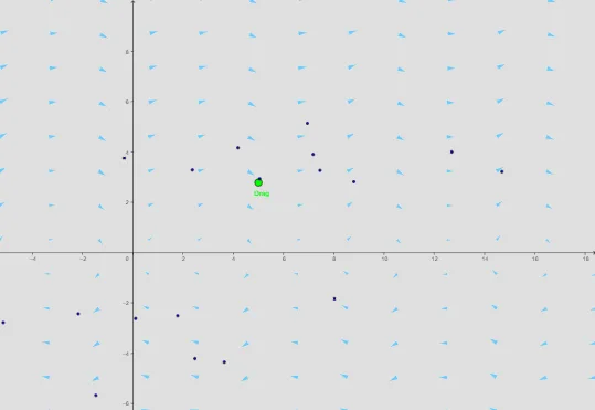
This example demonstrates the streamlines of a 2D velocity vector field, visually representing fluid motion trajectories. Core math concepts include vector fields, streamlines, and ordinary differential equation solving from calculus. Key GeoGebra commands used are SolveODE for solving ODEs to get streamlines, Sequence for trajectory sequences, and Textfield for displaying information. Dynamic demonstrations are achieved via timer and animate, with parameters controlled by sliders a, b, c, d. Suitable for university STEM students and learners interested in fluid mechanics and differential equations.
GeoGebra Commands & Parameters
SolveODE(G, F, x(B), y(B), -50, 0.01) → numericalIntegral2SolveODE(G, F, x(B), y(B), 80, 0.1) → numericalIntegral1Sequence(Sequence[Vector[(j, k), (j + (scale * F(j, k)), k + (scale * G(j, k)))], j, xmin, xmax, xstep], k, ymin, ymax, ystep) → FieldTextfield(F) → InputBox1Textfield(G) → InputBox2
AI Drawing Prompt Reference
Draw a 2D velocity vector field and its streamlines, where streamlines represent fluid motion trajectories. Use sliders to control parameters a, b, c, d, and solve differential equations with SolveODE to get streamlines. Generate the vector field with Sequence, and input functions for the x and y components of the velocity field in InputBox1 and InputBox2 respectively.
The prompt above was compiled from the original drawing commands and is for reference only.