
Lagrange Multipliers Example 6: Visualizing Constrained Optimization on a 3D Sur
Loading the math board and drawing, please wait…
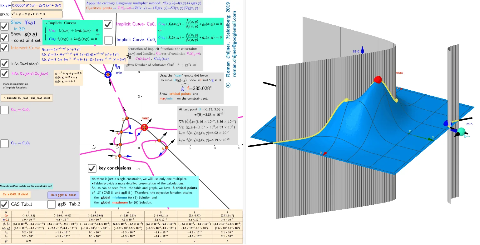
① This example demonstrates the method of Lagrange multipliers for solving constrained optimization problems, visually showing how the objective function and the constraint surface (a cylinder) are tangent at the extremum. ② Core mathematical concepts include multivariable extrema, Lagrange multipliers, gradient vectors, constraint surfaces, and the geometric relationship between tangent planes and normals. ③ Construction highlights: using GeoGebra commands such as CurveCartesian for parametric curves, Surface for the constraint surface, Vector for gradient vectors (Vf, Vg), Point for tangent points, Text and LaTeX for formulas, Slider (a, α) for interactive parameters, and Zip/Sequence for batch object generation, enabling dynamic exploration. ④ Suitable for university-level calculus or optimization courses, as well as advanced high school students interested in the geometric intuition behind Lagrange multipliers.
GeoGebra Commands & Parameters
Simplify(Derivative[f, y, 1]) → fy'Simplify(Derivative[f, x, 1]) → fx'LeftSide(Cu_g) → gSimplify(Derivative[g, y, 1]) → gy'Simplify(Derivative[g, x, 1]) → gx'Point(Cu_g) → BVector(B, B + UnitVector[Vector[B, Dg]] / 2) → u_gVector(B, B + UnitVector[Vector[B, Df]] / 2) → u_fAngle(u_g, u_f) → αLaTeX(f, true) → text8aLaTeX(Cu_g, true) → text8bLaTeX(Cu0_y, true) → txtCu0_yTextfield(f) → InputBox3Textfield(Cu_g) → InputBox4Zip((x(a), y(a), f(a)), a, Sequence[Point[Cu_g, t / n], t, 0, n]) → lg_1Textfield(n) → InputBox5CurveCartesian(t, (0.8 - t^(2)) / (t + 1), f(t, (0.8 - t^(2)) / (t + 1)), t, (-π), π) → q1Surface(t, (0.8 - t^(2)) / (t + 1), u, t, -3, 3, u, -0.1, 0.00001) → g1IndexOf(Min[z(l2f)], z(l2f)) → Indexmin2Element(l1, Indexmax1) → Amax1Element(l1, Indexmin1) → Amin1Element(l1f, Indexmax1) → Amax1_{3D}Element(l1f, Indexmin1) → Amin1_{3D}Element(l2f, Indexmin2) → Amin2_{3D}Element(l2, Indexmin2) → Amin2Element(l2, Indexmax2) → Amax2Element(l2f, Indexmax2) → Amax2_{3D}RotateText(text14, 90°) → text15TableText(Append["N", 1…Length[l1]], Append["\fgcolor{red}{Cp}", l1], Append["\fgcolor{blue}{f}(\fgcolor{red}{C_p })", l1fa], Append["(\dot{f_x},\dot{f_y})", l1xy'_fa], Append["(\dot{g_x},\dot{g_y})", l1xy'_ga], Append["λ_x", lλ1ax], Append["λ_y", lλ1ay], Append["\widehat{\dot{g}\dot{f}} ", lα1], "c|_") → tTab1TableText(Append["N", 1…Length[l2]], Append["\fgcolor{red}{Cp}", l2], Append["\fgcolor{blue}{f}(\fgcolor{red}{C_p })", l2fa], Append["(\dot{f_x},\dot{f_y})", l2xy'_fa], Append["(\dot{g_x},\dot{g_y})", l2xy'_ga], Append["λ_x", lλ2ax], Append["λ_y", lλ2ay], Append["\widehat{\dot{g}\dot{f}} ", lα2], "c|_") → tTab2Segment(B, C) → f_1Text("∇f", Point[u_f, 1]) → text25fText("∇g", Point[u_g, 1]) → text25gSimplify(fx'(x, y) - (gx'(x, y) * fy'(x, y) / gy'(x, y))) → Cu_xfSimplify(fy'(x, y) - (gy'(x, y) * fx'(x, y) / gx'(x, y))) → Cu_yfTextfield(txtCu01_x) → InputBox1Textfield(txtCu01_y) → InputBox2RemoveUndefined(Zip[Vector[c, c + UnitVector[a] / 2], a, l1xy'_f, c, l1]) → lvec1_fRemoveUndefined(Zip[Vector[c, c + UnitVector[a] / 2], a, l2xy'_f, c, l2]) → lvec2_fRemoveUndefined(Zip[Vector[c, c + UnitVector[a] / 2], a, l1xy'_g, c, l1]) → lvec1_gRemoveUndefined(Zip[Vector[c, c + UnitVector[a] / 2], a, l2xy'_g, c, l2]) → lvec2_gZip(Segment[a, b], a, l1, b, l1f) → l1segSequence(Text[i, l1(i) - (0.2, 0.1)], i, 1, lä1) → l1txtSequence(Text[i, l2(i) - (0.2, 0.1)], i, 1, lä2) → l2txtZip(Segment[a, b], a, l2, b, l2f) → l2seg
AI Drawing Prompt Reference
Create a 3D visualization of constrained optimization: a cylinder as the constraint surface, with a parametric curve on it representing feasible points. The objective function surface is tangent to the cylinder at extremum points. At each tangency point, draw two gradient vectors—one perpendicular to the objective level curve and one perpendicular to the constraint surface—and mark the angle between them. Show the projection of the objective function along the constraint curve, and place multiple sample points on the curve with short segments indicating gradient directions. Add text labels for gradients and function expressions, and include a table listing coordinates, function values, and gradient components for each sample point.
The prompt above was compiled from the original drawing commands and is for reference only.