
Lagrange Multipliers Example 4
Loading the math board and drawing, please wait…
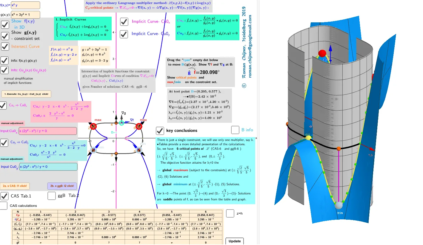
This example demonstrates finding extrema of a function subject to a constraint in 2D using the method of Lagrange multipliers. Key math concepts include vectors, derivatives, function optimization, and systems of linear equations. GeoGebra commands/objects used in construction are highlighted, such as Simplify, Point, Vector, Angle, LaTeX, Textfield, CurveCartesian, Segment, Text, RemoveUndefined, Element, Sequence. Suitable for university-level calculus and mathematical analysis courses to visually illustrate abstract optimization problems.
GeoGebra Commands & Parameters
Simplify(Derivative[f, y, 1]) → fy'Simplify(Derivative[f, x, 1]) → fx'LeftSide(Cu_g) → gSimplify(Derivative[g, y, 1]) → gy'Simplify(Derivative[g, x, 1]) → gx'Point(Cu_g) → BVector(B, B + UnitVector[Vector[B, Dg]] / 3) → u_gVector(B, B + UnitVector[Vector[B, Df]] / 3) → u_fAngle(u_g, u_f) → αLaTeX(f, true) → text8aLaTeX(Cu_g, true) → text8bTextfield(f) → InputBox3Textfield(Cu_g) → InputBox4Zip((x(a), y(a), f(a)), a, Sequence[Point[Cu_g, t / n], t, 0, n]) → lg_1Textfield(n) → InputBox5CurveCartesian(sqrt(t), sqrt((1 - t^(3)) / 3), f(sqrt(t), sqrt((1 - t^(3)) / 3)), t, 0, 1) → q1CurveCartesian((-sqrt(t)), sqrt((1 - t^(3)) / 3), f((-sqrt(t)), sqrt((1 - t^(3)) / 3)), t, 0, 1) → q2Surface((1 - (3 * t^(2)))^(1 / 6), t, u, t, -1 / sqrt(3), 1 / sqrt(3), u, -1.2, 1.2) → g1Surface((-(1 - (3 * t^(2)))^(1 / 6)), t, u, t, -1 / sqrt(3), 1 / sqrt(3), u, -1.2, 1.2) → g2CurveCartesian((-sqrt(t)), (-sqrt((1 - t^(3)) / 3)), f((-sqrt(t)), (-sqrt((1 - t^(3)) / 3))), t, 0, 1) → q1aCurveCartesian(sqrt(t), (-sqrt((1 - t^(3)) / 3)), f(sqrt(t), (-sqrt((1 - t^(3)) / 3))), t, 0, 1) → q2aRotateText(text3, 90°) → text5TableText(Append["N", 1…Length[l2]], Append["\fgcolor{red}{Cp}", l2], Append["\fgcolor{blue}{f}(\fgcolor{red}{C_p })", l2fa], Append["(\dot{f_x},\dot{f_y})", l2xy'_fa], Append["(\dot{g_x},\dot{g_y})", l2xy'_ga], Append["λ_x", lλ2ax], Append["λ_y", lλ2ay], Append["\widehat{\dot{g}\dot{f}} ", lα2], "c|_") → tTab2Zip(Text["(" + (SurdText[x(a)]) + "," + (SurdText[y(a)]) + ")", (0, 0), true, true], a, l2) → l2surdZip(Text["(" + (SurdText[x(a), {sqrt(2), sqrt(3), sqrt(5), sqrt(10), cbrt(2), cbrt(3), cbrt(5)}]) + "," + (SurdText[y(a), {sqrt(2), sqrt(3), sqrt(5), sqrt(10), cbrt(2), cbrt(3), cbrt(5)}]) + ")", (0, 0), true, true], a, l1) → l1surdTableText(Append["N", 1…Length[l1]], Append["\fgcolor{red}{Cp}", l1], Append["\fgcolor{blue}{f}(\fgcolor{red}{C_p })", l1fa], Append["(\dot{f_x},\dot{f_y})", l1xy'_fa], Append["(\dot{g_x},\dot{g_y})", l1xy'_ga], Append["λ_x", lλ1ax], Append["λ_y", lλ1ay], Append["\widehat{\dot{g}\dot{f}} ", lα1], "c|_") → tTab1Segment(B, C) → f_1Text("∇g", Point[u_g, 1]) → text25gText("∇f", Point[u_f, 1]) → text25fSimplify(fx'(x, y) - (gx'(x, y) * fy'(x, y) / gy'(x, y))) → Cu_xfSimplify(fy'(x, y) - (gy'(x, y) * fx'(x, y) / gx'(x, y))) → Cu_yfRemoveUndefined(Zip[Vector[c, c + UnitVector[a] / 3], a, l1xy'_f, c, l1]) → lvec1_fRemoveUndefined(Zip[Vector[c, c + UnitVector[a] / 3], a, l2xy'_f, c, l2]) → lvec2_fRemoveUndefined(Zip[Vector[c, c + UnitVector[a] / 3], a, l1xy'_g, c, l1]) → lvec1_gRemoveUndefined(Zip[Vector[c, c + UnitVector[a] / 3], a, l2xy'_g, c, l2]) → lvec2_gTextfield(txtCu01_x) → InputBox1Textfield(txtCu01_x) → InputBox2Element(l1, Indexmax1) → Amax1_1Element(l1, Indexmin1) → Amin1_1Element(l2, Indexmin2) → Amin2_1Zip(Segment[a, b], a, l1, b, l1f) → l1segSequence(Text[i, l1(i) - (0.2, 0.1)], i, 1, lä1) → l1txtSequence(Text[i, l2(i) - (0.2, 0.1)], i, 1, lä2) → l2txtZip(Segment[a, b], a, l2, b, l2f) → l2segElement(l1f, Indexmax1) → Amax13d_1Element(l2f, Indexmax2) → Amax23d_1Element(l1f, Indexmin1) → Amin13d_1Element(l2f, Indexmin2) → Amin23d_1Element(l1f, 5) → Amin13d_2Element(l1, 6) → Amax1_2Element(l2, 6) → Amax2_2Element(l2, Indexmax2) → Amax2_1Element(l1f, 6) → Amax13d_2Element(l2f, 6) → Amax23d_2Element(l2f, 5) → Amin23d_2Element(l1, 5) → Amin1_2Element(l2, 5) → Amin2_2
AI Drawing Prompt Reference
Visualize a 2D function optimization problem using Lagrange multipliers to find extrema. Include the function and constraint curves with their tangent vectors, gradient vectors, and the angle between them. Differentiate the function and constraint curves with colors, label key points and vectors, and present a table with coordinates, function values, gradient vectors, and Lagrange multipliers.
The prompt above was compiled from the original drawing commands and is for reference only.