
Lagrange Multiplier Method
Loading the math board and drawing, please wait…
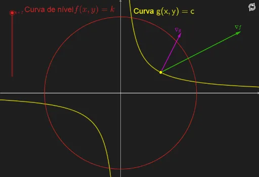
This GeoGebra example visually demonstrates the geometric meaning and calculation process of the Lagrange multiplier method for finding extrema of functions subject to constraints. It constructs the Lagrangian function, level curves, and constraint surfaces, illustrating how critical points are located where derivatives vanish. Key construction elements include points, vectors, equation systems, cylinder diagrams, and multiple text annotation objects, clearly showing the application of multivariable calculus in optimization. Suitable for advanced high school or university calculus courses as a teaching demonstration and self-study resource.
GeoGebra Commands & Parameters
Point(eq1) → CVector(C, C + (y(C), x(C))) → uVector(C, C + ((2 * x(C)), (2 * y(C)))) → v
AI Drawing Prompt Reference
Draw the geometric meaning of the Lagrange multiplier method, including a point C and two vectors u and v starting from C, pointing in the directions of (1,1) and (2x,2y) respectively. First, take a point C on equation eq1, then draw vector u from C to C+(y(C), x(C)), and draw vector v from C to C+(2*x(C), 2*y(C)), illustrating the critical points where the derivatives vanish under the constraint.
The prompt above was compiled from the original drawing commands and is for reference only.