
Intuitive Explorations of Inverse Trig Functions
Loading the math board and drawing, please wait…
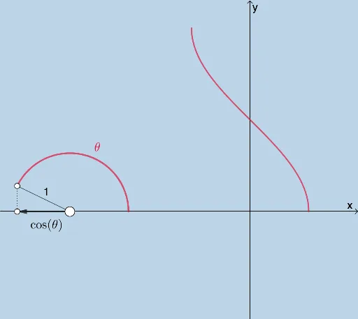
This example dynamically demonstrates the graphs and properties of inverse trigonometric functions, intuitively showing their domains, ranges, and geometric meanings. It involves core concepts like inverse trigonometric functions, trigonometric graphs, geometric transformations, and continuity. The construction utilizes GeoGebra commands and objects such as Rotate, OrthogonalLine, Intersect, Circle, Ray, etc. Suitable for high school and above mathematics learners to understand the intuitive concepts and properties of inverse trigonometric functions.
GeoGebra Commands & Parameters
Rotate(B, β, A) → B'_4OrthogonalLine(B'_4, xAxis) → j_1Intersect(j_1, xAxis) → JCircle(A, 1) → cRotate(B, α, A) → B'OrthogonalLine(B', xAxis) → iOrthogonalLine(B, xAxis) → jRay(A, B') → kSegment(A, B') → lIntersect(i, xAxis) → CRotate(C, If[0 < m ≤ 1, (m * π / 2), π / 2], A) → C'Dilate(A, If[1 < m ≤ 2, 2 - m, 0], D) → A'Vector(A, A') → uTranslate(C', u) → C''Rotate(C'', If[2 < m ≤ 3, ((-(m - 2)) * π / 2), ((-π)) / 2], D) → C'''Mirror(B, A) → B'_1Semicircle(B'_1, B) → pCircleArc(A, B, B') → qDilate(B, If[4 < m ≤ 5, 5 - m, 0], E) → B'_2Vector(B, B'_2) → vTranslate(c, v) → c'Translate(B', v) → B''Center(c') → FRotate(B'', If[4 < m ≤ 5, ((-(m - 4)) * α), (-α)], F) → B'''Segment(B, B'_2) → rCircleArc(F, B'_2, B''') → sDilate(B, If[6 < m ≤ 7, 7 - m, 0], C''') → B'_3Vector(B, B'_3) → wTranslate(B'_2, w) → GVector(A, C) → tVector(A, C') → u_1Vector(A', C'') → v_1Vector(D, C''') → w_1Vector(B, E) → a_1Vector(B'_3, G) → b_1Segment(B', C) → f_1OrthogonalLine(B, xAxis) → i_1Ray(A, B'_4) → g_1Intersect(i_1, g_1) → HSegment(A, B'_4) → h_1Vector(J, B'_4) → c_1Vector(B, H) → d_1Dilate(J, If[0 < m ≤ 1, 1 - m, 0], D) → J'Vector(J, J') → e_1Translate(B'_4, e_1) → IVector(J', I) → k_1Rotate(I, If[1 < m ≤ 2, ((-(m - 1)) * π / 2), ((-π)) / 2], D) → I'Vector(D, I') → l_1CircleArc(A, B'_4, B) → p_1CircleArc(A, B, B'_4) → q_1Dilate(B, If[3 < m ≤ 4, 4 - m, 0], L) → B'_5Vector(B, B'_5) → m_1Translate(c, m_1) → c'_1Center(c'_1) → NSegment(B, B'_5) → n_1Translate(B'_4, m_1) → PRotate(P, If[3 < m ≤ 4, ((-(m - 3)) * β), (-β)], N) → P'CircleArc(N, B'_5, P') → r_1Mirror(r_1, xAxis) → s_1Mirror(B, xAxis) → B'_6Mirror(B'_5, xAxis) → QSegment(B'_6, Q) → t_1Mirror(I, xAxis) → I'_1Mirror(B'_4, xAxis) → RMirror(I', D) → I''Mirror(q_1, xAxis) → c_2Mirror(A, xAxis) → A'_1Mirror(B'_4, xAxis) → SSegment(A'_1, S) → f_2Mirror(c_1, xAxis) → u_2Mirror(k_1, xAxis) → v_2Mirror(l_1, D) → w_2Dilate(B, If[5 < m ≤ 6, 6 - m, 0], I') → B'_7Vector(B, B'_7) → b_2Vector(B, P') → d_2Translate(P', b_2) → P''Translate(B, b_2) → B'_8Vector(B'_8, P'') → e_2Mirror(P', xAxis) → P''_1Dilate(B, If[5 < m ≤ 6, 6 - m, 0], I'') → B'_9Vector(B, B'_9) → g_2Vector(B, P''_1) → h_2Translate(P''_1, g_2) → MVector(B'_9, M) → i_2Mirror(B'_8, D) → OMirror(I', D) → I''_1Ray(A, H) → j_2Mirror(d_1, xAxis) → k_2Mirror(H, xAxis) → H'Mirror(A, xAxis) → A'_2Mirror(H, xAxis) → H'_1Ray(A'_2, H'_1) → l_2Dilate(B, If[0 < m ≤ 1, 1 - m, 0], D) → B'_{10}Vector(B, B'_{10}) → m_2Translate(H, m_2) → H'_2Translate(d_1, m_2) → n_2Translate(H', m_2) → H''Vector(B'_{10}, H'_2) → p_2Vector(B'_{10}, H'') → q_2Segment(A, H) → r_2Mirror(B, A) → B'_{11}Segment(A, B) → s_2Segment(A, H') → t_2Rotate(H'_2, If[1 < m ≤ 2, ((-(m - 1)) * π / 2), ((-π)) / 2], D) → TRotate(H'', If[1 < m ≤ 2, ((-(m - 1)) * π / 2), ((-π)) / 2], D) → H'''Vector(D, T) → u_3Vector(D, H''') → v_3Intersect(c, r_2, 1) → UIntersect(c, t_2, 1) → VCircleArc(A, B, U) → c_3CircleArc(A, V, B) → d_3Dilate(B, If[3 < m ≤ 4, 4 - m, 0], W) → B'_{12}Dilate(B, If[3 < m ≤ 4, 4 - m, 0], Z) → B'_{13}Vector(B, B'_{12}) → w_3Vector(B, B'_{13}) → a_3Translate(A, w_3) → A'_3Translate(A, a_3) → A'_4Translate(V, a_3) → V'Translate(U, w_3) → U'Rotate(U', If[3 < m ≤ 4, ((-(m - 3)) * β), (-β)], A'_3) → U''Rotate(V', If[3 < m ≤ 4, ((m - 3) * β), β], A'_4) → V''Segment(B, B'_{12}) → f_3Segment(B, B'_{13}) → g_3CircleArc(A'_3, B'_{12}, U'') → e_3CircleArc(A'_4, V'', B'_{13}) → h_3Vector(B, V'') → b_3Vector(B, U'') → i_3Dilate(B, If[5 < m ≤ 6, 6 - m, 0], T) → B'_{14}Vector(B, B'_{14}) → j_3Translate(U'', j_3) → U'''Vector(B'_{14}, U''') → k_3Dilate(B, If[5 < m ≤ 6, 6 - m, 0], H''') → B'_{15}Vector(B, B'_{15}) → l_3Translate(V'', l_3) → V'''Vector(B'_{15}, V''') → m_3
AI Drawing Prompt Reference
Draw a dynamic illustration of inverse trigonometric functions, showing their graphs, domains, ranges, and geometric meanings. Start with a circle and a ray, then construct the inverse trigonometric function graphs using rotations and perpendicular lines, marking key points and segments, and finally demonstrate geometric transformations and continuity.
The prompt above was compiled from the original drawing commands and is for reference only.