
Intuitive Derivative Graphing Exercise: REVAMPED!!!
Loading the math board and drawing, please wait…
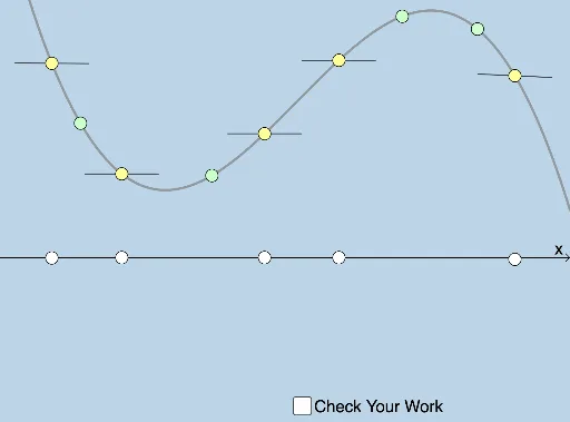
This example demonstrates how to graph derivative functions intuitively. It involves core math concepts like derivatives, tangent lines, function graphs, and optimization problems. Key GeoGebra commands used include FitPoly, Circle, Point, Intersect, Segment, Dilate, Vector, and Translate. Suitable for high school and above students to understand the geometric meaning of derivatives.
GeoGebra Commands & Parameters
FitPoly({A, B, C, D}, 3) → fCircle(A, 1) → cCircle(B, 1) → dCircle(C, 1) → eCircle(D, 1) → pPoint(f) → QPoint(a) → RCircle(Q, 1) → c_1Intersect(c_1, b) → S, TSegment(S, T) → f_1Point(f) → VPoint(f) → WPoint(f) → ZPoint(f) → A_1Point(g_1) → B_1Point(h_1) → C_1Point(i_1) → D_1Point(j_1) → E_1Circle(V, 1) → d_1Circle(W, 1) → e_1Circle(Z, 1) → p_1Circle(A_1, 1) → q_1Intersect(p_1, m_1) → F_1, G_1Intersect(q_1, n_1) → H_1, I_1Intersect(e_1, l_1) → J_1, K_1Intersect(d_1, k_1) → L_1, M_1Segment(L_1, M_1) → r_1Segment(J_1, K_1) → s_1Segment(F_1, G_1) → t_1Segment(H_1, I_1) → a_1Dilate(U, If[0 < u ≤ 1, 1 - u, 0], N_1) → U'Segment(U, U') → b_1Dilate(U, If[1 < u ≤ 2, 2 - u, 0], V) → U'_1Dilate(U, If[1 < u ≤ 2, 2 - u, 0], A) → U'_2Dilate(U, If[1 < u ≤ 2, 2 - u, 0], Q) → U'_3Dilate(U, If[1 < u ≤ 2, 2 - u, 0], W) → U'_5Dilate(U, If[1 < u ≤ 2, 2 - u, 0], C) → U'_6Dilate(U, If[1 < u ≤ 2, 2 - u, 0], Z) → U'_7Dilate(U, If[1 < u ≤ 2, 2 - u, 0], D) → U'_8Dilate(U, If[1 < u ≤ 2, 2 - u, 0], A_1) → U'_9Vector(U, U'_1) → vVector(U, U'_2) → wVector(U, U'_3) → u_1Vector(U, U'_5) → w_1Vector(U, U'_6) → u_2Vector(U, U'_7) → v_2Vector(U, U'_8) → w_2Vector(U, U'_9) → a_2Translate(U, w) → U'_{10}Translate(U', w) → U''Translate(U, u_1) → U'_{11}Translate(U', u_1) → U''_1Segment(U'_{11}, U''_1) → g_2Translate(U, v) → U'_{12}Translate(U', v) → U''_2Segment(U'_{12}, U''_2) → h_2Translate(U, w_1) → U'_{13}Translate(U', w_1) → U''_3Segment(U'_{13}, U''_3) → i_2Translate(U, v_2) → U'_{14}Translate(U', v_2) → U''_4Segment(U'_{14}, U''_4) → j_2Translate(U, w_2) → U'_{15}Translate(U', w_2) → U''_5Translate(U, a_2) → U'_{16}Translate(U', a_2) → U''_6Segment(U'_{16}, U''_6) → l_2Translate(U, w_1) → U'_{17}Translate(U', w_1) → U''_7Dilate(U, If[1 < u ≤ 2, 2 - u, 0], B) → U'_4Vector(U, U'_4) → v_1Translate(U, v_1) → U'_{18}Translate(U', v_1) → U''_8Dilate(U, If[1 < u ≤ 2, 2 - u, 0], C) → U'_{19}Vector(U, U'_6) → b_2Translate(U, b_2) → U'_{20}Translate(U', b_2) → U''_9Intersect(g, xAxis) → O_1Intersect(h, xAxis) → P_1Intersect(i, xAxis) → Q_1Intersect(xAxis, j) → R_1Intersect(g_1, xAxis) → S_1Intersect(h_1, xAxis) → T_1Intersect(i_1, xAxis) → U_1Intersect(a, xAxis) → V_1Vector(S_1, B_1) → c_2Vector(V_1, R) → e_2Vector(T_1, C_1) → r_2Vector(U_1, D_1) → t_2Dilate(S_1, If[3 < u ≤ 4, 4 - u, 0], U''_2) → W_1Dilate(O_1, If[3 < u ≤ 4, 4 - u, 0], U'') → E'Dilate(V_1, If[3 < u ≤ 4, 4 - u, 0], U''_1) → R'Dilate(P_1, If[3 < u ≤ 4, 4 - u, 0], U''_8) → Z_1Dilate(T_1, If[3 < u ≤ 4, 4 - u, 0], U''_7) → A_2Dilate(Q_1, If[3 < u ≤ 4, 4 - u, 0], U''_9) → B_2Dilate(U_1, If[3 < u ≤ 4, 4 - u, 0], U''_4) → C_2Dilate(R_1, If[3 < u ≤ 4, 4 - u, 0], U''_5) → D_2Dilate(R_1, If[3 < u ≤ 4, 4 - u, 0], U''_5) → E_2Dilate(F_2, If[3 < u ≤ 4, 4 - u, 0], U''_6) → G_2Translate(W_1, c_2) → H_2Vector(W_1, H_2) → v_3Translate(R', e_2) → R''Vector(R', R'') → a_3Translate(A_2, r_2) → J_2Vector(A_2, J_2) → c_3Translate(C_2, t_2) → L_2Vector(C_2, L_2) → e_3Vector(F_2, E_1) → g_3Translate(G_2, g_3) → N_2Vector(G_2, N_2) → h_3
AI Drawing Prompt Reference
Draw a function graph and its derivative graph to illustrate the geometric meaning of derivatives. First, fit a cubic polynomial as the original function. Then, mark several points on the function graph, draw circles centered at these points, and find their intersections with the function graph to get tangent lines. Next, draw several unit circles centered at points on the original function graph, intersect these circles with horizontal lines or the derivative function graph, and connect the intersection points to form approximate segments of the derivative graph. Finally, extend two line segments from the points on the original function graph to the left and right, representing the trend of function value changes.
The prompt above was compiled from the original drawing commands and is for reference only.