
Introductory Limit Problems: Functions, Geometry & Data Visualization
Loading the math board and drawing, please wait…
In collections
Calculus: Limits & Continuity
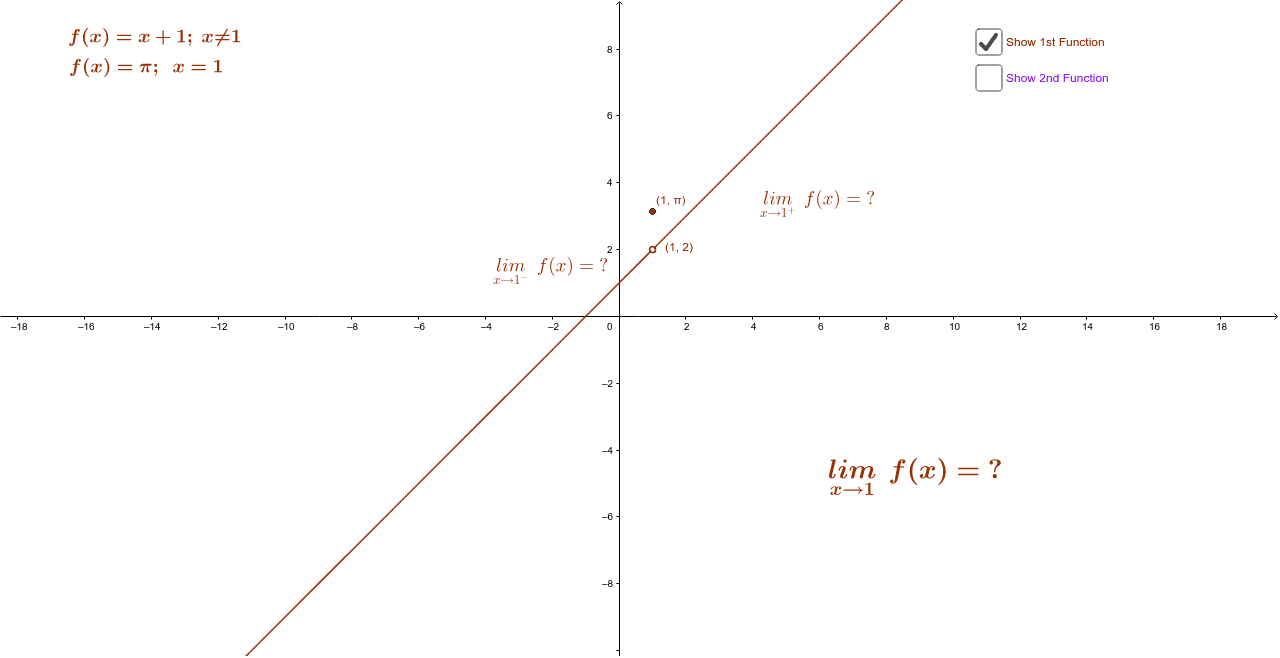
This GeoGebra example demonstrates fundamental limit concepts through multiple function graphs (f, g) with dynamic parameters (a, b) that show how functions approach specific values. Key mathematical concepts covered: definition of limits, function continuity, and one-sided limits. Construction details: plotting f and g using function commands, using sliders (a, b) to dynamically illustrate limit behavior, incorporating 3D objects (Cylinder, Cube) to visualize limits in geometric contexts, and using Histogram to show limit distributions of discrete data. Objects include points A, B, C for marking key positions and text elements (text1-6) for mathematical explanations. Suitable for high school calculus introduction courses or as visual teaching aids for college-level limit concepts, helping students build intuitive understanding of limits.
GeoGebra Commands & Parameters
f(x) = If[(-Infinity) ≤ x ≤ 0.95, x + 1]g(x) = If[1.05 ≤ x ≤ Infinity, x + 1]Point A(1.0, 2.0)Point B(1.0, 3.141592653589793)Point C(0.0, 6.0)h(x) = If[(-Infinity) ≤ x ≤ (-0.1), ((3 + x)^(2) - 9) / x]p(x) = If[0.1 ≤ x ≤ Infinity, ((3 + x)^(2) - 9) / x]Boolean a(true)Boolean b(false)
AI Drawing Prompt Reference
Draw two functions f(x) = x + 1 (for x from -∞ to 0.95) and g(x) = x + 1 (for x from 1.05 to ∞), and mark points A(1,2), B(1,3.14), and C(0,6). Use dynamic parameters a and b to illustrate the behavior of function limits, and show geometric contexts of limits with cylinders and cubes. Finally, use a histogram to display the limit distribution of discrete data.
The prompt above was compiled from the original drawing commands and is for reference only.