
Introduction to y = mx + c
Loading the math board and drawing, please wait…
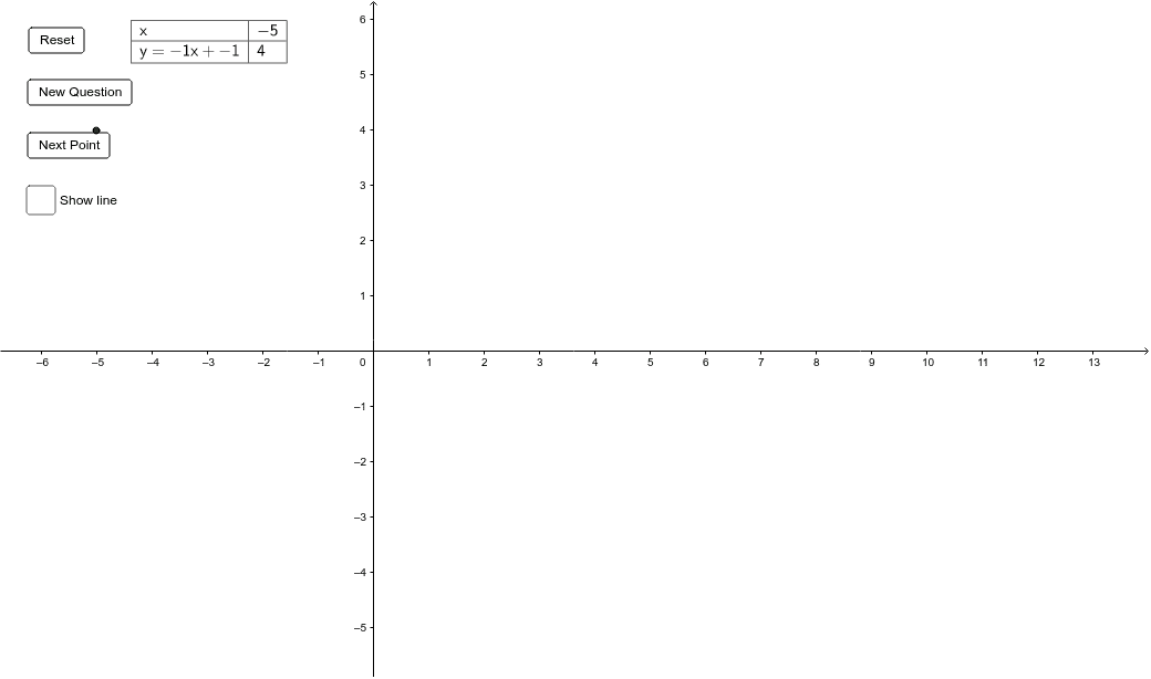
This example demonstrates the basic concept and graphical representation of the linear equation y = mx + c. Key math concepts include slope (m), y-intercept (c), and the representation of lines in a coordinate system. Construction highlights the use of GeoGebra commands Random, Sequence, Append, TableText and objects n, m, c, f, list1, button1, button2, button3, list2, list3, text1, a. Suitable for middle school and above students learning analytical geometry and function graphs.
GeoGebra Commands & Parameters
Random(-3, 3) → mRandom(-3, 3) → cSequence((i, f(i)), i, -5, n) → list1Append("x", Sequence[i + "", i, -5, n]) → list2Append("y = " + m + "x + " + c, Sequence[f(i) + "", i, -5, n]) → list3TableText({list2, list3}, "h_|") → text1
AI Drawing Prompt Reference
Draw a line with a slope between -2 and 2 and a y-intercept between -3 and 3. Generate points for x values from -5 to 5 and show their corresponding y values. Display the x-axis and the equation y=mx+c below the graph.
The prompt above was compiled from the original drawing commands and is for reference only.