
Introduction to Normal Distribution with Hand-Span Data
Loading the math board and drawing, please wait…
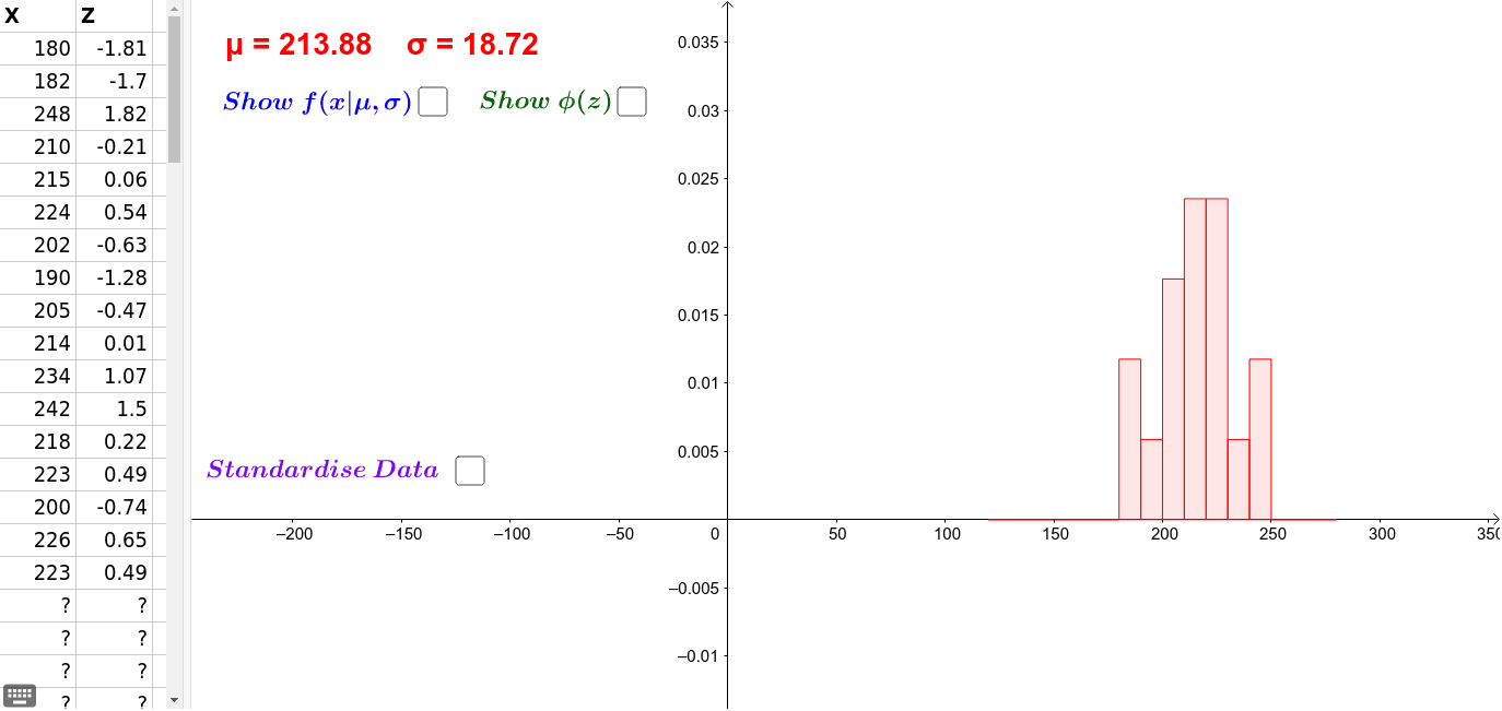
This example demonstrates fitting a normal distribution curve to real-world hand-span data. Key concepts include mean, standard deviation, probability density, and histograms. Construction utilizes GeoGebra commands like Mean, Histogram, and Textfield, processing data from list1 with parameters μ and σ. Ideal for high school or college statistics classes to visualize data distribution patterns.
GeoGebra Commands & Parameters
RemoveUndefined({A2, A3, A4, A5, A6, A7, A8, A9, A10, A11, A12, A13, A14, A15, A16, A17, A18, A20, A21, A22, A23, A24, A25, A26, A27, A28, A29, A30, A31, A32, A33, A34, A35, A36}) → list1Mean(list1) → aRemoveUndefined({B2, B3, B4, B5, B6, B7, B8, B9, B10, B11, B12, B13, B14, B15, B16, B17, B18, B20, B21, B22, B23, B24, B25, B26, B27, B28, B29, B30, B31, B32, B33, B34, B35, B36}) → list2Histogram(list3, list1, true, 1 / Length[list1]) → cHistogram((list3 - a) / b, list2, true, 1 / Length[list2]) → fTextfield(μ) → InputBox1Textfield(σ) → InputBox2