
Exploring the Normal Distribution
Loading the math board and drawing, please wait…
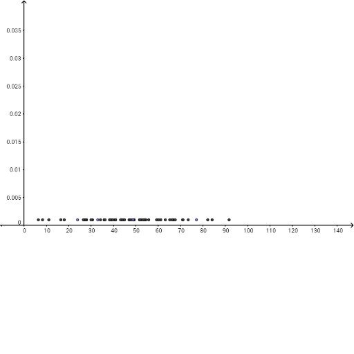
This example demonstrates the characteristics of the normal distribution, involving concepts such as random variables, mean, and standard deviation. Using GeoGebra commands like Segment, Point, Histogram, etc., it visually illustrates the graphical and statistical properties of the normal distribution. Suitable for high school mathematics education and learning.
GeoGebra Commands & Parameters
Segment((0, 0.001), (100, 0.001)) → aPoint(a) → APoint(a) → BPoint(a) → CPoint(a) → DPoint(a) → EPoint(a) → FPoint(a) → GPoint(a) → HPoint(a) → IPoint(a) → JPoint(a) → KPoint(a) → LPoint(a) → MPoint(a) → NPoint(a) → OPoint(a) → PPoint(a) → QPoint(a) → RPoint(a) → SPoint(a) → TPoint(a) → UPoint(a) → VPoint(a) → WPoint(a) → ZPoint(a) → A_1Point(a) → B_1Point(a) → C_1Point(a) → D_1Point(a) → E_1Point(a) → F_1Point(a) → G_1Point(a) → H_1Point(a) → I_1Point(a) → J_1Point(a) → K_1Point(a) → L_1Point(a) → M_1Point(a) → N_1Point(a) → O_1Point(a) → P_1Point(a) → Q_1Point(a) → R_1Point(a) → S_1Point(a) → T_1Point(a) → U_1Point(a) → V_1Point(a) → W_1Point(a) → Z_1Point(a) → A_2Point(a) → B_2Point(a) → C_2Point(a) → D_2Point(a) → E_2Point(a) → F_2Point(a) → G_2Point(a) → H_2Point(a) → I_2Point(a) → J_2Point(a) → K_2Point(a) → L_2Histogram({0, 10, 20, 30, 40, 50, 60, 70, 80, 90, 100}, B1:B60, true, 0.016666666666666666) → cMean(B1:B60) → meanSD(B1:B60) → sdBoxPlot(0.03, 0.001, mean - sd, mean, mean, mean, mean + sd) → dNormal(mean, sd, x) → gSegment((mean, 0), (mean, 0.02)) → hBoxPlot(0.033, 0.001, mean - (2 * sd), mean, mean, mean, mean + (2 * sd)) → eBoxPlot(0.036, 0.001, mean - (3 * sd), mean, mean, mean, mean + (3 * sd)) → fBoxPlot(0.025, 0.001, B1:B60) → bPolygon((105, 0.01), (115, 0.01), (115, 0.0116667), (105, 0.0116667)) → poly2, s, t, a_1, b_1NormalQuantilePlot(B1:B60) → list1
AI Drawing Prompt Reference
Draw a horizontal line from 0 to 100, then place 26 equally spaced points on this line to illustrate the graphical and statistical properties of the normal distribution.
The prompt above was compiled from the original drawing commands and is for reference only.