Approximating a Binomial Distribution using a Normal Distribution (2.04d, 2.04h)

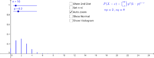
This GeoGebra example demonstrates how the probability mass function of a binomial distribution can be approximated by a normal distribution curve when the number of trials n is large and the success probability p is moderate. The core mathematical concept is the application of the central limit theorem to approximate a discrete distribution with a continuous one, involving binomial distribution, normal distribution, probability histograms, and density curve fitting. Construction details: the BinomialDist command generates binomial probabilities, Sequence builds lists, BarChart plots the probability histogram, and Normal draws the normal density curve. Objects include n, p, a, list1, list2, b, n', p', list3, list4, c, d, e, text1, text2, f, g, text3, h, q, i, j, k, and text4, allowing dynamic adjustment of parameters and display of approximation errors. Suitable for high school or college statistics courses explaining the normal approximation conditions (np≥5 and n(1-p)≥5) and continuity correction, as well as for exploring how approximation accuracy varies with n and p.