
Intersection of Two Parametric Curves via Implicit Curves with Graphical and Num
Loading the math board and drawing, please wait…
In collections
Solution of Systems of nonlinear Equations
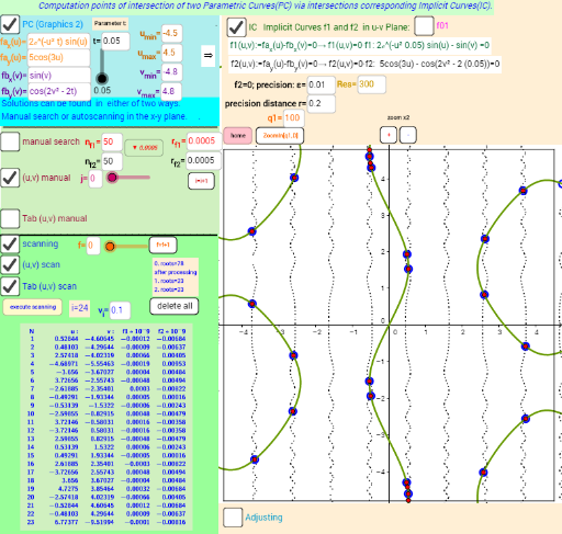
① This example demonstrates how to find all intersection points of two parametric curves by converting them into corresponding implicit curves, then using GeoGebra's CAS capabilities for both graphical and numerical solutions. ② Core mathematical concepts include parametric curves, implicit curves, intersection solving, numerical computation (CAS), and geometric visualization. ③ Construction highlights: from the summary, commands such as ImplicitCurve, Intersect, PolyLine, Point, PathParameter, ClosestPoint, Sequence, Zip, TableText are used; objects include sliders (r_a, r_b), text fields, and dynamic lists (listxyres1) to manage results. ④ Suitable for advanced high school or undergraduate courses in analytic geometry and calculus, as well as for mathematical experimentation, helping students understand the relationship between parametric and implicit representations and numerical solution techniques.
GeoGebra Commands & Parameters
ImplicitCurve(f1(x, y)) → aIntersect(Circle[D, r_a], OrthogonalLine[D, Segment[D, ClosestPoint[a, D]]], 2) → Hzz2ImplicitCurve(f2(x, y)) → bIntersect(Circle[D, r_b], OrthogonalLine[D, Segment[D, ClosestPoint[b, D]]], 1) → Z1_bIntersect(Circle[D, r_b], OrthogonalLine[D, Segment[D, ClosestPoint[b, D]]], 2) → Z2_bIntersect(Circle[D, r_a], OrthogonalLine[D, Segment[D, ClosestPoint[a, D]]], 1) → Z1_aPolyLine(Zip[ClosestPoint[b, B], B, Z1_b + ((Z2_b - Z1_b) / n_b * Sequence[i, i, 0, n_b])]) → polZbPolyLine(Zip[ClosestPoint[a, B], B, Z1_a + ((Z2_a - Z1_a) / n_a * Sequence[i, i, 0, n_a])]) → polZaElement({Intersect[polZa, polZb]}, 1) → PZPoint(a) → B_aPathParameter(B_a) → Pf1BTextfield(Nn) → InputBox4Textfield(e) → InputBox5Textfield(x_{min}) → InputBox6Textfield(x_{max}) → InputBox7Textfield(y_{min}) → InputBox8Textfield(y_{max}) → InputBox9Polygon((x_{min}, y_{min}), (x_{max}, y_{min}), (x_{max}, y_{max}), (x_{min}, y_{max})) → poly1, g1_s, g2_s, g3_s, s4_sTextfield(α) → InputBox2Length(lr1) → llr1Length(lf2) → llf2Textfield(r) → InputBox16CurveCartesian(fa_x(u), fa_y(u), u, x_{min}, x_{max}) → a_cCurveCartesian(fb_x(v), fb_y(v), v, y_{min}, y_{max}) → b_cElement(lr1, i_{manual}) → C_tElement(lgr2_bscan, f) → B_{xy}Length(lf1) → llf1Textfield(fa_x) → InputBox17Textfield(fa_y) → InputBox18Textfield(fb_x) → InputBox19Textfield(fb_y) → InputBox20Textfield(n_a) → InputBox21Textfield(n_b) → InputBox22Textfield(r_a) → InputBox23Textfield(q) → InputBox24PolyLine(Z1_a + ((Z2_a - Z1_a) / n_a * Sequence[i, i, 0, n_a])) → poly2_aaPolyLine(Z1_b + ((Z2_b - Z1_b) / n_b * Sequence[i, i, 0, n_b])) → poly2_bbPoint(poly2_aa, e1) → R_aPoint(poly2_bb, e2) → R_bClosestPoint(a, R_a) → R'_aClosestPoint(b, R_b) → R'_bLength(R'_a - R'_b) → dmaxmins2If(Defined[PZ], If[fza2 < fzb2, (f1za2, f2za2), (f1zb2, f2zb2)], (NaN, NaN)) → errorz2If(Defined[PZ], If[fza2 < fzb2, R'_a, R'_b], (NaN, NaN)) → Pz2If(ca, PZ, Pz2) → PZ0If(ca, f11, x(errorz2)) → f110If(ca, f22, y(errorz2)) → f220Textfield(r_b) → InputBox13Textfield(α) → InputBox11Element(roots0, f) → ASequence((fa_x(x(Element[lr1, i])), fa_y(x(Element[lr1, i]))), i, 1, llr1) → lgr2_aSequence((fb_x(y(Element[lr1, i])), fb_y(y(Element[lr1, i]))), i, 1, llr1) → lr2_bZip((((abs(x(a - b) / x(a)) * 100), (abs(y(a - b) / y(a)) * 100)) * 1000000000), a, lgr2_a, b, lr2_b) → lgr2Element(lgr2_a, i_{manual}) → Cxy_tTextfield(t) → InputBox1Textfield(f) → InputBox3Textfield(i_{manual}) → Eingabefeld1Textfield(q2) → Eingabefeld2ImplicitCurve(f01(x, y)) → cIf(Length[listxyres1] ≟ 0 ∨ (i > m1), F, Element[listxyres1, i]) → BLength(lr2) → llr2TableText({Join[{{"N"}, Sequence[i, i, 1, Length[roots0]]}], Join[{{""}, Sequence["→", i, 1, f]}], Join[{{" u:"}, x(roots0)}], Join[{{" v:"}, y(roots0)}], Join[{{"f1*10^-9"}, lf1_{Pr}2}], Join[{{"f2* 10^-9"}, lf2_{Pr}2}]}, "vr") → Text2TableText({Join[{{"N"}, Sequence[i, i, 1, Length[roots0]]}], Join[{{""}, Sequence["→", i, 1, f]}], Join[{{"(x,y)_a"}, lgr2_ascan}], Join[{{"(x,y)_b"}, lgr2_bscan}], Join[{{"(δx,δy) %*10^-9"}, lgr2scan}]}, "vr") → text12aTableText({Join[{{"N"}, Sequence[i, i, 1, llr1]}], Join[{{""}, Sequence["→", i, 1, i_{manual}]}], Join[{{"u:"}, x(lr1)}], Join[{{"v:"}, y(lr1)}], Join[{{"f1* 10^-9"}, lf1}], Join[{{"f2* 10^-9"}, lf2}]}, "vr") → text8Intersect(Circle[D, r_a], OrthogonalLine[D, Segment[D, ClosestPoint[a, D]]], 1) → Hzz1TableText({Join[{{"N"}, Sequence[i, i, 1, llr1]}], Join[{{""}, Sequence["→", i, 1, i_{manual}]}], Join[{{"(x,y)_a"}, lgr2_a}], Join[{{"(x,y)_b"}, lr2_b}], Join[{{"(δx,δy) %*10-9"}, lgr2}]}, "vr") → text12rTextfield(v_i) → InputBox10
AI Drawing Prompt Reference
Draw the intersection points of two parametric curves by first converting them into implicit curves. Use sliders to adjust parameters and observe changes in intersection points. Draw paths of intersection points and display their coordinates. Set the coordinate axis range and show the parametric equations of the curves.
The prompt above was compiled from the original drawing commands and is for reference only.