
Intersection of Cylinder and Cone
Loading the math board and drawing, please wait…
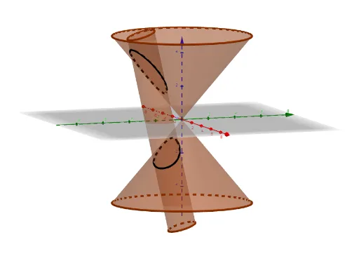
This example demonstrates the intersection of a cylinder and a cone. Key mathematical concepts include solid geometry and coordinate geometry. Using GeoGebra commands such as Point, Cylinder, Cone, and CurveCartesian, the intersection can be constructed. Suitable for high school mathematics education or learning.
GeoGebra Commands & Parameters
Point({s, t, -5}) → APoint({s, t, 5}) → BCylinder(Point[{s, (t * cos(θ)) - (h_{Zylinder} * sin(θ)), (t * sin(θ)) + (h_{Zylinder} * cos(θ))}], Point[{s, (t * cos(θ)) + (h_{Zylinder} * sin(θ)), (t * sin(θ)) - (h_{Zylinder} * cos(θ))}], r) → d_2, d_2, d_3, d_4Cone(Point[{0, 0, h_{Kegel}}], Point[{0, 0, 0}], (h_{Kegel} * R)) → k, k_2, k_3Cone(Point[{0, 0, (-h_{Kegel})}], Point[{0, 0, 0}], (h_{Kegel} * R)) → m, m_2, m_3CurveCartesian(f_{up}(η), (cos(θ) * η) - ((sin(θ) * 1 / (((sin((2 * θ)) * (1 + R^(2))) * η))) * (f_{up}(η)^(2) + ((1 - R^(2)) * η^(2)))), (sin(θ) * η) + ((cos(θ) * 1 / (((sin((2 * θ)) * (1 + R^(2))) * η))) * (f_{up}(η)^(2) + ((1 - R^(2)) * η^(2)))), η, t - r, t + r) → γ_uCurveCartesian(f_{down}(η), (cos(θ) * η) - ((sin(θ) * 1 / (((sin((2 * θ)) * (1 + R^(2))) * η))) * (f_{down}(η)^(2) + ((1 - R^(2)) * η^(2)))), (sin(θ) * η) + ((cos(θ) * 1 / (((sin((2 * θ)) * (1 + R^(2))) * η))) * (f_{down}(η)^(2) + ((1 - R^(2)) * η^(2)))), η, t - r, t + r) → γ_dCurveCartesian(0, (t * (-sin(θ))), (t * cos(θ)), t, -24, 24) → cCoefficients(Polynomial[D_0]) → L_0If(Element[L_0, 2]^(2) - ((4 * Element[L_0, 1]) * Element[L_0, 3]) < 0, t, (1 / ((2 * Element[L_0, 1])) * ((-Element[L_0, 2]) - (Element[L_0, 2]^(2) - ((4 * Element[L_0, 1]) * Element[L_0, 3]))^(0.5)))) → η_{01}If(Element[L_0, 2]^(2) - ((4 * Element[L_0, 1]) * Element[L_0, 3]) < 0, t, (1 / ((2 * Element[L_0, 1])) * ((-Element[L_0, 2]) + (Element[L_0, 2]^(2) - ((4 * Element[L_0, 1]) * Element[L_0, 3]))^(0.5)))) → η_{02}CurveCartesian((r^(2) - (η - t)^(2))^(0.5), η, (1 / R * (((2 * t) * η) - t^(2) + r^(2))^(0.5)), η, t - r, t + r) → δ_{uu}CurveCartesian((-(r^(2) - (η - t)^(2))^(0.5)), η, (1 / R * (((2 * t) * η) - t^(2) + r^(2))^(0.5)), η, t - r, t + r) → δ_{du}CurveCartesian((r^(2) - (η - t)^(2))^(0.5), η, (-1 / R * (((2 * t) * η) - t^(2) + r^(2))^(0.5)), η, t - r, t + r) → δ_{ud}CurveCartesian((-(r^(2) - (η - t)^(2))^(0.5)), η, (-1 / R * (((2 * t) * η) - t^(2) + r^(2))^(0.5)), η, t - r, t + r) → δ_{dd}CurveCartesian(f_{up}(η), (η * cos(θ)) - ((sin(θ) * 1 / ((2 * a))) * ((((1 + R^(2)) * sin((2 * θ))) * η) + D_{sup}(η)^(0.5))), (η * sin(θ)) + ((cos(θ) * 1 / ((2 * a))) * ((((1 + R^(2)) * sin((2 * θ))) * η) + D_{sup}(η)^(0.5))), η, t - r, t + r) → γ_{uu}CurveCartesian(f_{up}(η), (η * cos(θ)) - ((sin(θ) * 1 / ((2 * a))) * ((((1 + R^(2)) * sin((2 * θ))) * η) - D_{sup}(η)^(0.5))), (η * sin(θ)) + ((cos(θ) * 1 / ((2 * a))) * ((((1 + R^(2)) * sin((2 * θ))) * η) - D_{sup}(η)^(0.5))), η, t - r, t + r) → γ_{ud}CurveCartesian(f_{down}(η), (η * cos(θ)) - ((sin(θ) * 1 / ((2 * a))) * ((((1 + R^(2)) * sin((2 * θ))) * η) + D_{sdown}(η)^(0.5))), (η * sin(θ)) + ((cos(θ) * 1 / ((2 * a))) * ((((1 + R^(2)) * sin((2 * θ))) * η) + D_{sdown}(η)^(0.5))), η, t - r, t + r) → γ_{du}CurveCartesian(f_{down}(η), (η * cos(θ)) - ((sin(θ) * 1 / ((2 * a))) * ((((1 + R^(2)) * sin((2 * θ))) * η) - D_{sdown}(η)^(0.5))), (η * sin(θ)) + ((cos(θ) * 1 / ((2 * a))) * ((((1 + R^(2)) * sin((2 * θ))) * η) - D_{sdown}(η)^(0.5))), η, t - r, t + r) → γ_{dd}
AI Drawing Prompt Reference
Describe a 3D geometric figure formed by the intersection of a cylinder and a cone. The cylinder and cone intersect in a curve or surface. The figure includes a cylinder and a cone, possibly with parallel or intersecting axes. The intersection forms a closed curve or multiple curves. This figure is useful for illustrating 3D geometry concepts.
The prompt above was compiled from the original drawing commands and is for reference only.